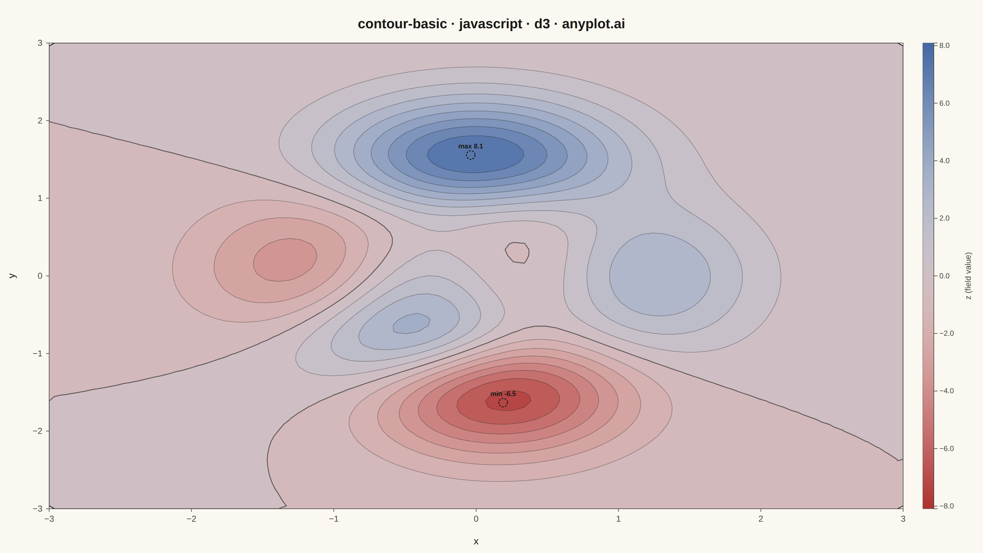
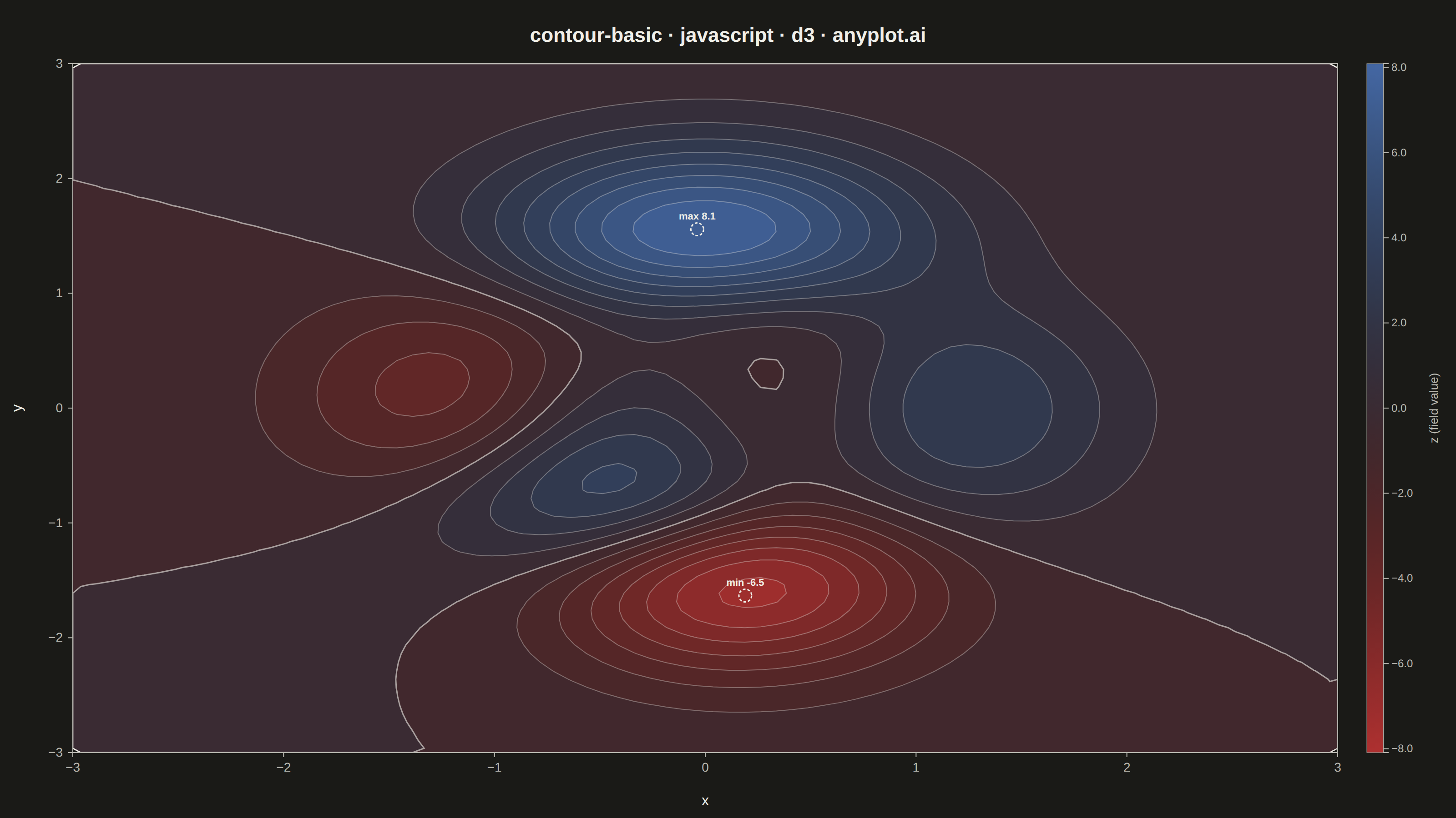
The same plot in 14 other libraries — JavaScript: Chart.js, Apache ECharts, Highcharts, MUI X Charts; Python: Altair, Bokeh, lets-plot, Matplotlib, Plotly, plotnine, Pygal, Seaborn; R: ggplot2; Julia: Makie.jl. Compare all 15 side by side: Basic Contour Plot in Python, R, Julia and JavaScript.
A contour plot displays isolines (level curves) of a 2D scalar field, connecting points of equal value across a surface. It transforms 3D data into an intuitive 2D representation, making it easy to identify regions of high and low values, gradients, and patterns. Contour plots are essential for visualizing continuous surfaces where the relationship between X, Y coordinates and a Z value needs to be understood.
// anyplot.ai
// contour-basic: Basic Contour Plot
// Library: d3 7.9.0 | JavaScript 22.23.0
// Quality: 88/100 | Created: 2026-06-25

const t = window.ANYPLOT_TOKENS;
const { width, height } = window.ANYPLOT_SIZE;
const margin = { top: 70, right: 130, bottom: 72, left: 80 };
const iw = width - margin.left - margin.right;
const ih = height - margin.top - margin.bottom;

// --- Data: "peaks" function on [-3, 3] × [-3, 3], produces both positive and negative values ---
const nx = 80, ny = 80;
const values = new Float64Array(nx * ny);
for (let j = 0; j < ny; j++) {
  for (let i = 0; i < nx; i++) {
    const x = -3 + 6 * i / (nx - 1);
    const y = 3 - 6 * j / (ny - 1); // j=0 → y=3 (top), j=ny-1 → y=-3 (bottom)
    const x2 = x * x, y2 = y * y;
    values[j * nx + i] =
      3 * (1 - x) * (1 - x) * Math.exp(-x2 - (y + 1) * (y + 1)) -
      10 * (x / 5 - x * x2 - y * y2 * y2) * Math.exp(-x2 - y2) -
      (1 / 3) * Math.exp(-(x + 1) * (x + 1) - y2);
  }
}
const vmin = d3.min(values);
const vmax = d3.max(values);
const absMax = Math.max(Math.abs(vmin), Math.abs(vmax));

// Find grid indices of global max and min for focal-point annotations
let maxIdx = 0, minIdx = 0;
for (let k = 1; k < values.length; k++) {
  if (values[k] > values[maxIdx]) maxIdx = k;
  if (values[k] < values[minIdx]) minIdx = k;
}
const peakX = -3 + 6 * (maxIdx % nx) / (nx - 1);
const peakY = 3 - 6 * Math.floor(maxIdx / nx) / (ny - 1);
const troughX = -3 + 6 * (minIdx % nx) / (nx - 1);
const troughY = 3 - 6 * Math.floor(minIdx / nx) / (ny - 1);

// --- SVG mount ---
const svg = d3.select("#container").append("svg").attr("width", width).attr("height", height);
const defs = svg.append("defs");

defs.append("clipPath").attr("id", "pc")
  .append("rect").attr("width", iw).attr("height", ih);

const g = svg.append("g").attr("transform", `translate(${margin.left},${margin.top})`);

// --- Contour generation ---
const numLevels = 18;
const thresholds = d3.range(numLevels + 1).map(i => -absMax + 2 * absMax * i / numLevels);
const contoursData = d3.contours().size([nx, ny]).thresholds(thresholds)(values);

// Projection: grid space [0..nx] × [0..ny] → plot area [0..iw] × [0..ih]
const geoProj = d3.geoTransform({
  point: function(px, py) { this.stream.point(px * iw / nx, py * ih / ny); }
});
const pathGen = d3.geoPath(geoProj);

// Diverging Imprint colormap: red (negative) → near-bg → blue (positive)
const colorScale = d3.scaleSequential(d3.interpolateRgbBasis(t.div)).domain([-absMax, absMax]);

// --- Filled contour bands (clipped to plot area) ---
const cg = g.append("g").attr("clip-path", "url(#pc)");

cg.selectAll(".cf").data(contoursData).join("path")
  .attr("class", "cf").attr("d", pathGen)
  .attr("fill", d => colorScale(d.value)).attr("stroke", "none");

// --- Contour isolines: increased visibility; zero-crossing isoline emphasized ---
const step = 2 * absMax / numLevels;
cg.selectAll(".cl").data(contoursData).join("path")
  .attr("class", "cl").attr("d", pathGen)
  .attr("fill", "none")
  .attr("stroke", t.ink)
  .attr("stroke-width", d => Math.abs(d.value) < step ? 1.5 : 1.0)
  .attr("stroke-opacity", d => Math.abs(d.value) < step ? 0.6 : 0.35);

// --- Plot border (all four sides — standard for contour plots) ---
g.append("rect").attr("width", iw).attr("height", ih)
  .attr("fill", "none").attr("stroke", t.inkSoft).attr("stroke-width", 1);

// --- Axes ---
const xScale = d3.scaleLinear().domain([-3, 3]).range([0, iw]);
const yScale = d3.scaleLinear().domain([3, -3]).range([0, ih]);

const xAx = g.append("g").attr("transform", `translate(0,${ih})`)
  .call(d3.axisBottom(xScale).ticks(7).tickSize(5).tickPadding(6));
xAx.select(".domain").remove();
xAx.selectAll(".tick line").attr("stroke", t.inkSoft);
xAx.selectAll(".tick text").attr("fill", t.inkSoft).style("font-size", "14px");

const yAx = g.append("g")
  .call(d3.axisLeft(yScale).ticks(7).tickSize(5).tickPadding(6));
yAx.select(".domain").remove();
yAx.selectAll(".tick line").attr("stroke", t.inkSoft);
yAx.selectAll(".tick text").attr("fill", t.inkSoft).style("font-size", "14px");

// --- Axis labels ---
g.append("text")
  .attr("x", iw / 2).attr("y", ih + 58)
  .attr("text-anchor", "middle")
  .attr("fill", t.ink).style("font-size", "16px")
  .text("x");

g.append("text")
  .attr("transform", `translate(-56,${ih / 2}) rotate(-90)`)
  .attr("text-anchor", "middle")
  .attr("fill", t.ink).style("font-size", "16px")
  .text("y");

// --- Colorbar ---
const cbW = 18, cbX = iw + 32;
const cbGrad = defs.append("linearGradient").attr("id", "cbg")
  .attr("x1", "0%").attr("y1", "100%").attr("x2", "0%").attr("y2", "0%");
for (let s = 0; s <= 30; s++) {
  const f = s / 30;
  cbGrad.append("stop")
    .attr("offset", `${(f * 100).toFixed(1)}%`)
    .attr("stop-color", colorScale(-absMax + 2 * absMax * f));
}

g.append("rect")
  .attr("x", cbX).attr("y", 0).attr("width", cbW).attr("height", ih)
  .style("fill", "url(#cbg)").attr("stroke", t.inkSoft).attr("stroke-width", 0.5);

const cbScale = d3.scaleLinear().domain([-absMax, absMax]).range([ih, 0]);
const cbAx = g.append("g").attr("transform", `translate(${cbX + cbW},0)`)
  .call(d3.axisRight(cbScale).ticks(6).tickFormat(d3.format(".1f")));
cbAx.selectAll(".tick text").attr("fill", t.inkSoft).style("font-size", "12px");
cbAx.selectAll(".tick line").attr("stroke", t.inkSoft);
cbAx.select(".domain").attr("stroke", t.inkSoft);

g.append("text")
  .attr("transform", `translate(${cbX + cbW + 60},${ih / 2}) rotate(-90)`)
  .attr("text-anchor", "middle")
  .attr("fill", t.inkSoft).style("font-size", "13px")
  .text("z (field value)");

// --- Focal-point annotations: global max and min ---
const focalPts = [
  { x: peakX,   y: peakY,   label: `max ${values[maxIdx].toFixed(1)}` },
  { x: troughX, y: troughY, label: `min ${values[minIdx].toFixed(1)}` },
];
cg.selectAll(".fp-ring").data(focalPts).join("circle")
  .attr("class", "fp-ring")
  .attr("cx", d => xScale(d.x)).attr("cy", d => yScale(d.y))
  .attr("r", 7).attr("fill", "none")
  .attr("stroke", t.ink).attr("stroke-width", 1.5).attr("stroke-dasharray", "3,2");

cg.selectAll(".fp-lbl").data(focalPts).join("text")
  .attr("class", "fp-lbl")
  .attr("x", d => xScale(d.x)).attr("y", d => yScale(d.y) - 11)
  .attr("text-anchor", "middle")
  .attr("fill", t.ink).style("font-size", "11px").style("font-weight", "600")
  .text(d => d.label);

// --- Title ---
svg.append("text")
  .attr("x", width / 2).attr("y", 46)
  .attr("text-anchor", "middle").attr("fill", t.ink)
  .style("font-size", "22px").style("font-weight", "600")
  .text("contour-basic · javascript · d3 · anyplot.ai");
Runnable source as JSON, for any HTTP client: https://api.anyplot.ai/specs/contour-basic/d3/code. Any spec id and library id listed in llms-full.txt fit the same URL shape; every URL below is complete and callable.
{
  "spec_id": "contour-basic",
  "language": "javascript",
  "library": "d3",
  "page": "https://anyplot.ai/contour-basic/javascript/d3",
  "hub": "https://anyplot.ai/contour-basic",
  "code_json": "https://api.anyplot.ai/specs/contour-basic/d3/code",
  "spec_json": "https://api.anyplot.ai/specs/contour-basic",
  "render_light_png": "https://storage.googleapis.com/anyplot-images/plots/contour-basic/javascript/d3/plot-light.png",
  "render_dark_png": "https://storage.googleapis.com/anyplot-images/plots/contour-basic/javascript/d3/plot-dark.png",
  "interactive_light_html": "https://storage.googleapis.com/anyplot-images/plots/contour-basic/javascript/d3/plot-light.html",
  "interactive_dark_html": "https://storage.googleapis.com/anyplot-images/plots/contour-basic/javascript/d3/plot-dark.html",
  "quality_score": 88.0,
  "license": "MIT",
  "guide": "https://anyplot.ai/llms.txt"
}
Part of Basic Contour Plot on anyplot.ai.