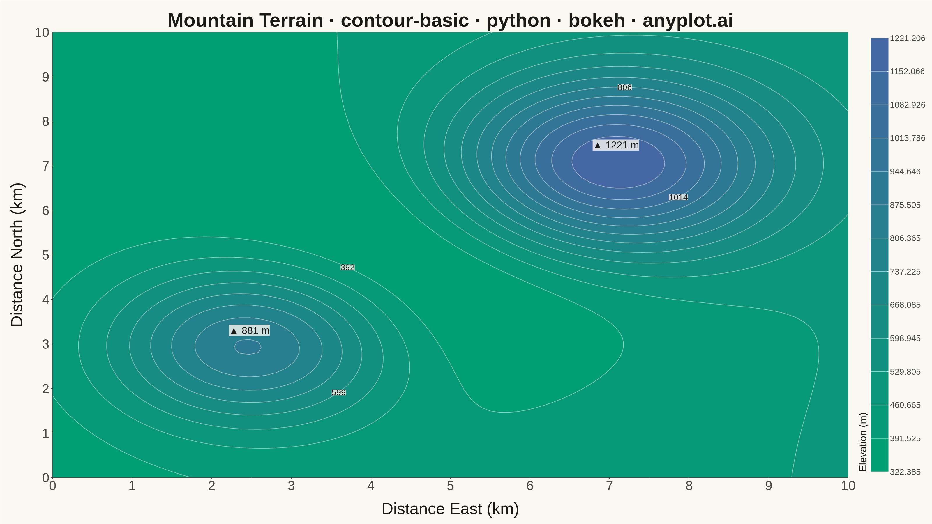
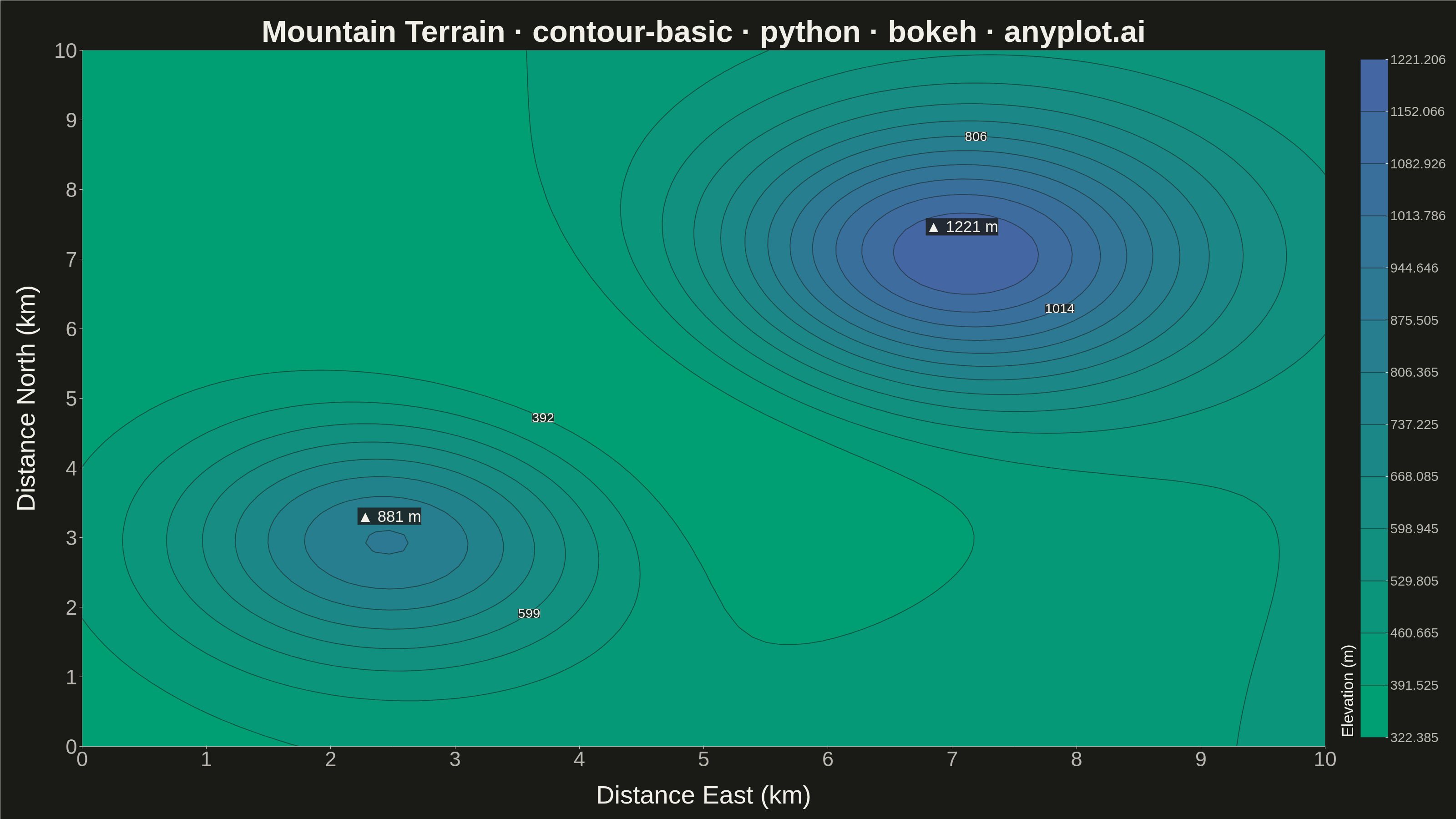
A contour plot displays isolines (level curves) of a 2D scalar field, connecting points of equal value across a surface. It transforms 3D data into an intuitive 2D representation, making it easy to identify regions of high and low values, gradients, and patterns. Contour plots are essential for visualizing continuous surfaces where the relationship between X, Y coordinates and a Z value needs to be understood.
""" anyplot.ai
contour-basic: Basic Contour Plot
Library: bokeh 3.9.1 | Python 3.13.14
Quality: 93/100 | Updated: 2026-06-25
"""

import os
import sys
import time
from pathlib import Path


# bokeh.py shadows the installed bokeh package — remove current dir from path
sys.path = [p for p in sys.path if p not in ("", os.getcwd())]

import numpy as np
from bokeh.io import output_file, save
from bokeh.models import HoverTool, Label, LinearColorMapper
from bokeh.plotting import figure
from selenium import webdriver
from selenium.webdriver.chrome.options import Options


THEME = os.getenv("ANYPLOT_THEME", "light")
PAGE_BG = "#FAF8F1" if THEME == "light" else "#1A1A17"
ELEVATED_BG = "#FFFDF6" if THEME == "light" else "#242420"
INK = "#1A1A17" if THEME == "light" else "#F0EFE8"
INK_SOFT = "#4A4A44" if THEME == "light" else "#B8B7B0"

# Imprint sequential palette: brand green (#009E73) → blue (#4467A3) — 256 stops
_r0, _g0, _b0 = 0x00, 0x9E, 0x73
_r1, _g1, _b1 = 0x44, 0x67, 0xA3
ANYPLOT_SEQ256 = [
    "#{:02X}{:02X}{:02X}".format(
        round(_r0 + (_r1 - _r0) * t / 255), round(_g0 + (_g1 - _g0) * t / 255), round(_b0 + (_b1 - _b0) * t / 255)
    )
    for t in range(256)
]

# Data — simulated topographic elevation map of a 10km x 10km mountain region
x = np.linspace(0, 10, 90)
y = np.linspace(0, 10, 90)
X, Y = np.meshgrid(x, y)

elevation = (
    850 * np.exp(-((X - 7) ** 2 + (Y - 7) ** 2) / 4.0)
    + 550 * np.exp(-((X - 2.5) ** 2 + (Y - 3) ** 2) / 3.0)
    - 180 * np.exp(-((X - 5) ** 2 + (Y - 5) ** 2) / 8.0)
    + 12 * X
    + 350
)

levels = np.linspace(elevation.min(), elevation.max(), 14)

# Locate the two peaks for annotations
_ne_iy, _ne_ix = np.unravel_index(elevation.argmax(), elevation.shape)
x_ne, y_ne = float(x[_ne_ix]), float(y[_ne_iy])
ne_peak_elev = int(round(float(elevation[_ne_iy, _ne_ix])))

_sw_elev = np.where((X < 5) & (Y < 6), elevation, 0)
_sw_iy, _sw_ix = np.unravel_index(_sw_elev.argmax(), _sw_elev.shape)
x_sw, y_sw = float(x[_sw_ix]), float(y[_sw_iy])
sw_peak_elev = int(round(float(elevation[_sw_iy, _sw_ix])))

# Title — 62 chars, below 67-char baseline
title = "Mountain Terrain · contour-basic · python · bokeh · anyplot.ai"

# Plot — canonical 3200×1800 landscape canvas
W, H = 3200, 1800
p = figure(
    width=W,
    height=H,
    title=title,
    x_axis_label="Distance East (km)",
    y_axis_label="Distance North (km)",
    toolbar_location=None,
    x_range=(0, 10),
    y_range=(0, 10),
    match_aspect=True,
    min_border_bottom=160,
    min_border_left=180,
    min_border_top=110,
    min_border_right=50,
)

contour = p.contour(
    x=X, y=Y, z=elevation, levels=levels, fill_color=ANYPLOT_SEQ256, line_color=PAGE_BG, line_width=2, line_alpha=0.45
)

colorbar = contour.construct_color_bar(
    title="Elevation (m)",
    title_text_font_size="26pt",
    title_text_color=INK,
    title_text_font_style="normal",
    title_standoff=20,
    major_label_text_font_size="22pt",
    major_label_text_color=INK_SOFT,
    background_fill_color=PAGE_BG,
    border_line_color=None,
    width=60,
    padding=20,
)
p.add_layout(colorbar, "right")

# Invisible image renderer — enables HoverTool elevation readout in the HTML artifact
_mapper = LinearColorMapper(palette=ANYPLOT_SEQ256, low=elevation.min(), high=elevation.max())
_img_r = p.image(image=[elevation], x=0, y=0, dw=10, dh=10, color_mapper=_mapper, alpha=0)
p.add_tools(
    HoverTool(
        renderers=[_img_r], tooltips=[("Position", "($x{0.1f} km E, $y{0.1f} km N)"), ("Elevation", "@image{0} m")]
    )
)

# Contour level labels — every 3rd level labels key isolines (spec: "label when practical")
for _i in (1, 4, 7, 10):
    _level_val = levels[_i]
    _diff = np.abs(elevation - _level_val)
    # Exclude borders and the right-side colorbar zone (x > ~8)
    _diff[:4, :] = np.inf
    _diff[-4:, :] = np.inf
    _diff[:, :4] = np.inf
    _diff[:, -18:] = np.inf
    _iy, _ix = np.unravel_index(_diff.argmin(), _diff.shape)
    if np.isfinite(_diff[_iy, _ix]):
        p.add_layout(
            Label(
                x=float(x[_ix]),
                y=float(y[_iy]),
                text=f"{int(round(_level_val))}",
                text_font_size="22pt",
                text_color=INK,
                text_align="center",
                text_baseline="middle",
                background_fill_color=PAGE_BG,
                background_fill_alpha=0.8,
                border_line_color=INK_SOFT,
                border_line_alpha=0.4,
            )
        )

# Summit annotations — storytelling focal points for the two elevation peaks
for _x_pk, _y_pk, _elev_pk in ((x_ne, y_ne, ne_peak_elev), (x_sw, y_sw, sw_peak_elev)):
    p.add_layout(
        Label(
            x=_x_pk,
            y=_y_pk,
            text=f"▲ {_elev_pk} m",
            text_font_size="26pt",
            text_color=INK,
            text_align="center",
            text_baseline="bottom",
            x_offset=0,
            y_offset=40,
            background_fill_color=PAGE_BG,
            background_fill_alpha=0.8,
            border_line_color=None,
        )
    )

# Typography — sized for 3200×1800 canvas
p.title.text_font_size = "50pt"
p.title.text_font_style = "bold"
p.title.text_color = INK
p.title.align = "center"

p.xaxis.axis_label_text_font_size = "42pt"
p.yaxis.axis_label_text_font_size = "42pt"
p.xaxis.axis_label_text_font_style = "normal"
p.yaxis.axis_label_text_font_style = "normal"
p.xaxis.major_label_text_font_size = "34pt"
p.yaxis.major_label_text_font_size = "34pt"
p.xaxis.axis_label_standoff = 28
p.yaxis.axis_label_standoff = 28

# Theme-adaptive chrome
p.background_fill_color = PAGE_BG
p.border_fill_color = PAGE_BG
p.outline_line_color = None  # frameless — cleaner minimalist look

p.xaxis.axis_label_text_color = INK
p.yaxis.axis_label_text_color = INK
p.xaxis.major_label_text_color = INK_SOFT
p.yaxis.major_label_text_color = INK_SOFT
p.xaxis.axis_line_color = INK_SOFT
p.yaxis.axis_line_color = INK_SOFT
p.xaxis.major_tick_line_color = INK_SOFT
p.yaxis.major_tick_line_color = INK_SOFT
p.xaxis.minor_tick_line_color = None
p.yaxis.minor_tick_line_color = None

# Filled contour covers the plot area — disable grid to avoid noise
p.xgrid.grid_line_color = None
p.ygrid.grid_line_color = None

p.xaxis.ticker.desired_num_ticks = 10
p.yaxis.ticker.desired_num_ticks = 8

# Save HTML (interactive catalog artifact)
output_file(f"plot-{THEME}.html", title="contour-basic · bokeh · anyplot.ai")
save(p)

# Screenshot with headless Chrome — CDP device override ensures exact W×H pixel output
opts = Options()
for arg in (
    "--headless=new",
    "--no-sandbox",
    "--disable-dev-shm-usage",
    "--disable-gpu",
    f"--window-size={W},{H}",
    "--hide-scrollbars",
):
    opts.add_argument(arg)
driver = webdriver.Chrome(options=opts)
driver.execute_cdp_cmd(
    "Emulation.setDeviceMetricsOverride", {"width": W, "height": H, "deviceScaleFactor": 1, "mobile": False}
)
driver.get(f"file://{Path(f'plot-{THEME}.html').resolve()}")
time.sleep(3)
driver.save_screenshot(f"plot-{THEME}.png")
driver.quit()
Runnable source as JSON, for any HTTP client: https://api.anyplot.ai/specs/contour-basic/bokeh/code. Any spec id and library id listed in llms-full.txt fit the same URL shape; every URL below is complete and callable.
{
  "spec_id": "contour-basic",
  "language": "python",
  "library": "bokeh",
  "page": "https://anyplot.ai/contour-basic/python/bokeh",
  "hub": "https://anyplot.ai/contour-basic",
  "code_json": "https://api.anyplot.ai/specs/contour-basic/bokeh/code",
  "spec_json": "https://api.anyplot.ai/specs/contour-basic",
  "render_light_png": "https://storage.googleapis.com/anyplot-images/plots/contour-basic/python/bokeh/plot-light.png",
  "render_dark_png": "https://storage.googleapis.com/anyplot-images/plots/contour-basic/python/bokeh/plot-dark.png",
  "interactive_light_html": "https://storage.googleapis.com/anyplot-images/plots/contour-basic/python/bokeh/plot-light.html",
  "interactive_dark_html": "https://storage.googleapis.com/anyplot-images/plots/contour-basic/python/bokeh/plot-dark.html",
  "quality_score": 93.0,
  "license": "MIT",
  "guide": "https://anyplot.ai/llms.txt"
}
Part of Basic Contour Plot on anyplot.ai.