The same plot in 14 other libraries — JavaScript: D3.js, Apache ECharts, Highcharts, MUI X Charts; Python: Altair, Bokeh, lets-plot, Matplotlib, Plotly, plotnine, Pygal, Seaborn; R: ggplot2; Julia: Makie.jl. Compare all 15 side by side: Pharmacological Dose-Response Curve in Python, R, Julia and JavaScript.
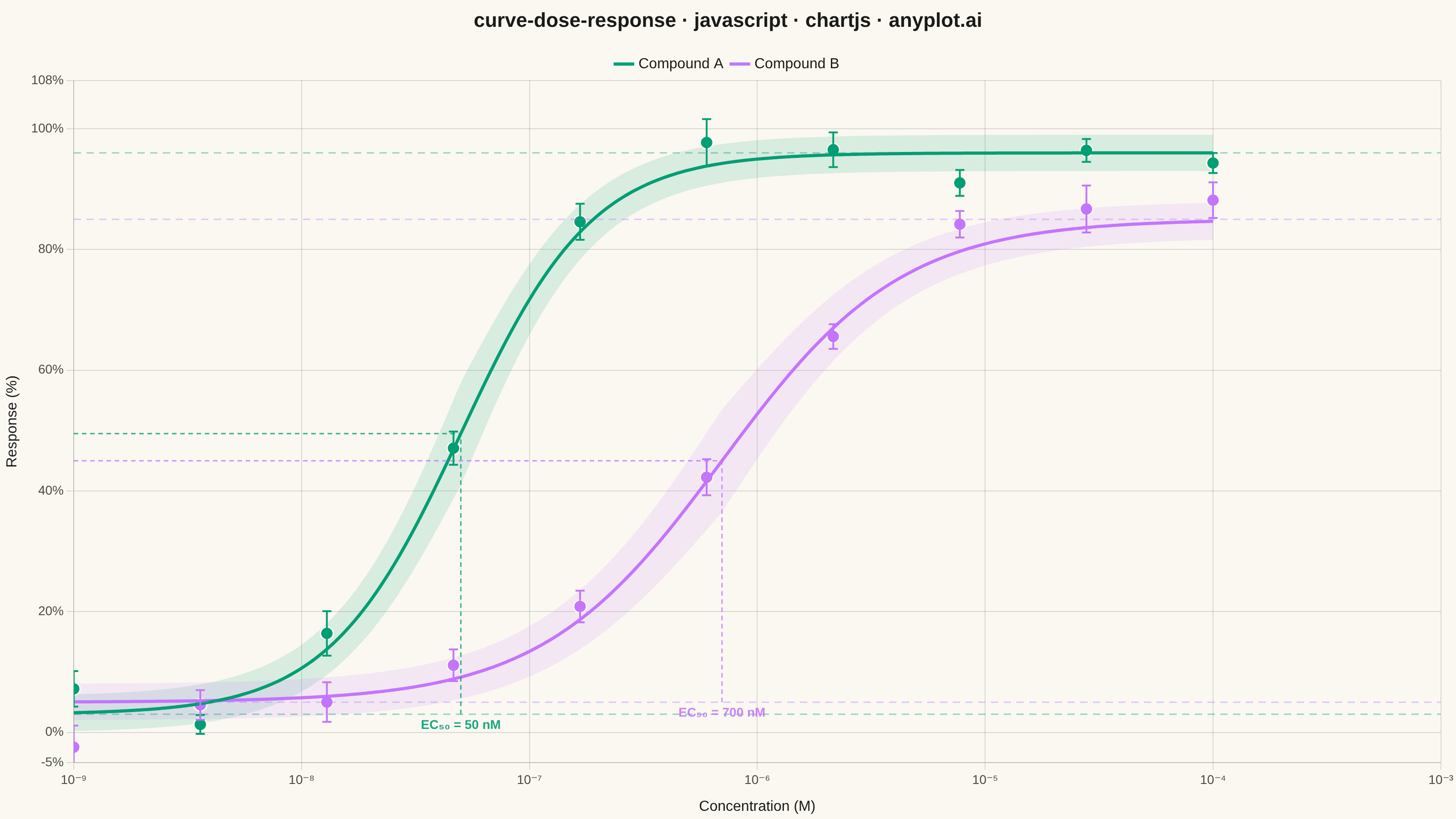
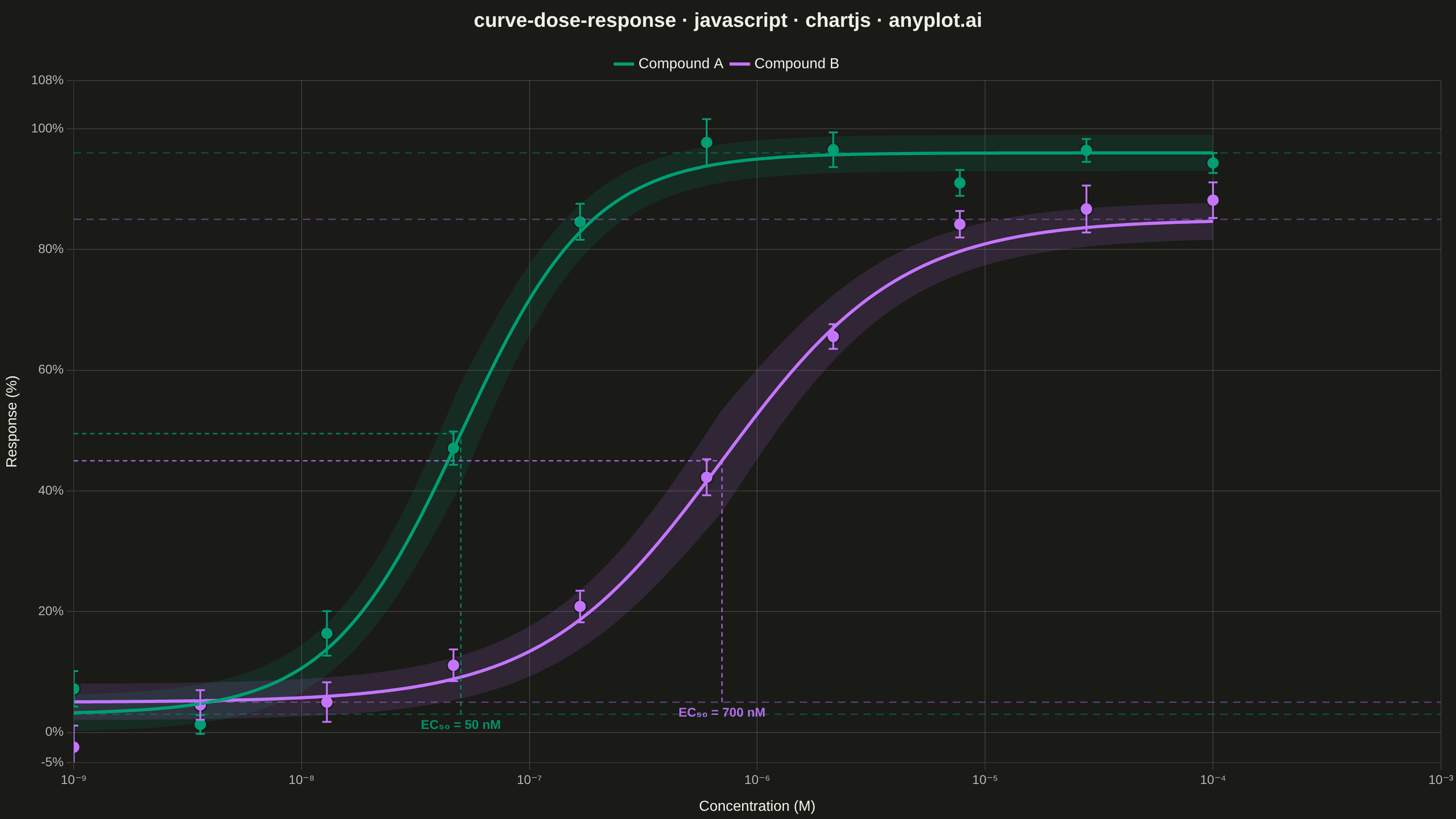
A sigmoidal dose-response curve that plots biological response against drug concentration on a logarithmic x-axis, fitted using a four-parameter logistic (4PL) model. This visualization is essential for determining drug potency metrics such as EC50 (half-maximal effective concentration) or IC50 (half-maximal inhibitory concentration), Hill slope steepness, and upper/lower response asymptotes. It enables rapid visual comparison of compound efficacy and is a standard tool in pharmacological analysis.
// anyplot.ai
// curve-dose-response: Pharmacological Dose-Response Curve
// Library: chartjs 4.4.7 | JavaScript 22.22.3
// Quality: 91/100 | Created: 2026-06-24

const t = window.ANYPLOT_TOKENS;

// 4-parameter logistic (4PL) sigmoid
function fourPL(c, bot, top, ec50, hill) {
  return bot + (top - bot) / (1 + Math.pow(ec50 / c, hill));
}

// log-spaced concentration array
function logSpace(lo, hi, n) {
  const a = Math.log10(lo), b = Math.log10(hi);
  return Array.from({ length: n }, (_, i) => Math.pow(10, a + (b - a) * i / (n - 1)));
}

// seeded LCG pseudo-random for reproducible noise
let _seed = 42;
function rand() { _seed = (_seed * 1664525 + 1013904223) >>> 0; return _seed / 0x100000000; }
function randN() { return Math.sqrt(-2 * Math.log(rand() + 1e-15)) * Math.cos(2 * Math.PI * rand()); }

// Compound parameters — Imprint palette positions 0 and 1
const COMPOUNDS = [
  { name: "Compound A", color: t.palette[0], bot: 3,  top: 96, ec50: 5e-8, hill: 1.5 },
  { name: "Compound B", color: t.palette[1], bot: 5,  top: 85, ec50: 7e-7, hill: 1.1 },
];

// Concentration grids
const DATA_C  = logSpace(1e-9, 1e-4, 10);
const CURVE_C = logSpace(1e-9, 1e-4, 200);

// 95% CI half-width: peaks near the inflection point of the sigmoid
function ciHW(c, cpd) {
  const r   = fourPL(c, cpd.bot, cpd.top, cpd.ec50, cpd.hill);
  const mid  = (cpd.bot + cpd.top) / 2;
  const half = (cpd.top - cpd.bot) / 2;
  return 3 + (1 - Math.abs(r - mid) / half) * 5.5;
}

// Generate observed data: true response + Gaussian noise + SEM
const CPD_DATA = COMPOUNDS.map(cpd => ({
  ...cpd,
  pts: DATA_C.map(c => {
    const tr = fourPL(c, cpd.bot, cpd.top, cpd.ec50, cpd.hill);
    return { c, r: tr + randN() * 2.8, sem: 1.5 + rand() * 2.5 };
  }),
}));

// EC50 formatter: prefer nM below 1000, μM above
function fmtEC50(ec50) {
  const nM = ec50 * 1e9;
  return nM < 1000
    ? `EC₅₀ = ${Math.round(nM)} nM`
    : `EC₅₀ = ${+(nM / 1000).toFixed(2)} μM`;
}

// Unicode superscript digits for log-axis tick labels
function toSup(n) {
  const MAP = { "0":"⁰","1":"¹","2":"²","3":"³","4":"⁴","5":"⁵","6":"⁶","7":"⁷","8":"⁸","9":"⁹","-":"⁻" };
  return String(n).split("").map(c => MAP[c] || c).join("");
}

// ---- Datasets: fitted curve (in legend) + observed scatter (hidden) ----
const datasets = CPD_DATA.flatMap((cpd, ci) => [
  {
    label: cpd.name,
    data: CURVE_C.map(c => ({ x: c, y: fourPL(c, cpd.bot, cpd.top, cpd.ec50, cpd.hill) })),
    showLine: true,
    pointRadius: 0,
    borderColor: cpd.color,
    backgroundColor: "transparent",
    borderWidth: 3.5,
    tension: 0.3,
  },
  {
    label: `_pts${ci}`,
    data: cpd.pts.map(p => ({ x: p.c, y: p.r })),
    showLine: false,
    pointRadius: 7,
    pointHoverRadius: 9,
    borderColor: t.pageBg,
    backgroundColor: cpd.color,
    borderWidth: 1.5,
  },
]);

// ---- CI Band Plugin: drawn before datasets so bands sit behind the curves ----
const ciBandPlugin = {
  id: "ciBands",
  beforeDatasetsDraw(chart) {
    const { ctx, chartArea: A, scales: { x: xS, y: yS } } = chart;
    ctx.save();
    ctx.beginPath();
    ctx.rect(A.left, A.top, A.right - A.left, A.bottom - A.top);
    ctx.clip();

    CPD_DATA.forEach(cpd => {
      ctx.fillStyle = cpd.color + "22"; // ~13% alpha fill
      ctx.beginPath();
      CURVE_C.forEach((c, i) => {
        const px = xS.getPixelForValue(c);
        const py = yS.getPixelForValue(fourPL(c, cpd.bot, cpd.top, cpd.ec50, cpd.hill) + ciHW(c, cpd));
        i === 0 ? ctx.moveTo(px, py) : ctx.lineTo(px, py);
      });
      [...CURVE_C].reverse().forEach(c => {
        ctx.lineTo(
          xS.getPixelForValue(c),
          yS.getPixelForValue(fourPL(c, cpd.bot, cpd.top, cpd.ec50, cpd.hill) - ciHW(c, cpd))
        );
      });
      ctx.closePath();
      ctx.fill();
    });

    ctx.restore();
  },
};

// ---- Overlay Plugin: asymptotes, EC50 lines, and SEM error bars ----
const overlayPlugin = {
  id: "overlay",
  afterDatasetsDraw(chart) {
    const { ctx, chartArea: A, scales: { x: xS, y: yS } } = chart;
    ctx.save();
    ctx.beginPath();
    ctx.rect(A.left, A.top, A.right - A.left, A.bottom - A.top);
    ctx.clip();

    // Top and bottom asymptote dashed lines
    CPD_DATA.forEach(cpd => {
      [cpd.bot, cpd.top].forEach(level => {
        ctx.save();
        ctx.strokeStyle = cpd.color;
        ctx.lineWidth = 1.5;
        ctx.globalAlpha = 0.4;
        ctx.setLineDash([8, 6]);
        const yPx = yS.getPixelForValue(level);
        ctx.beginPath();
        ctx.moveTo(A.left, yPx);
        ctx.lineTo(A.right, yPx);
        ctx.stroke();
        ctx.restore();
      });
    });

    // EC50 dashed reference lines (vertical + horizontal) and text label
    CPD_DATA.forEach(cpd => {
      const mid    = (cpd.bot + cpd.top) / 2;
      const xEC    = xS.getPixelForValue(cpd.ec50);
      const yMid   = yS.getPixelForValue(mid);
      const yBotPx = yS.getPixelForValue(cpd.bot);

      ctx.save();
      ctx.strokeStyle = cpd.color;
      ctx.lineWidth = 1.5;
      ctx.globalAlpha = 0.8;
      ctx.setLineDash([5, 4]);

      // Vertical: bottom asymptote → midpoint
      ctx.beginPath();
      ctx.moveTo(xEC, yBotPx);
      ctx.lineTo(xEC, yMid);
      ctx.stroke();

      // Horizontal: left axis → EC50
      ctx.beginPath();
      ctx.moveTo(A.left, yMid);
      ctx.lineTo(xEC, yMid);
      ctx.stroke();
      ctx.restore();

      // EC50 text label just below the vertical reference line
      ctx.save();
      ctx.fillStyle = cpd.color;
      ctx.globalAlpha = 0.9;
      ctx.font = "bold 14px sans-serif";
      ctx.textAlign = "center";
      ctx.textBaseline = "top";
      ctx.fillText(fmtEC50(cpd.ec50), xEC, yBotPx + 5);
      ctx.restore();
    });

    // SEM error bars on observed data points
    CPD_DATA.forEach((cpd, ci) => {
      const meta = chart.getDatasetMeta(ci * 2 + 1);
      if (!meta || meta.hidden) return;

      ctx.save();
      ctx.strokeStyle = cpd.color;
      ctx.lineWidth = 2;
      ctx.setLineDash([]);

      meta.data.forEach((el, i) => {
        const xPx = el.x;
        const { r, sem } = cpd.pts[i];
        const yT  = yS.getPixelForValue(r + sem);
        const yB  = yS.getPixelForValue(r - sem);
        const cap = 5;

        ctx.beginPath(); ctx.moveTo(xPx, yT); ctx.lineTo(xPx, yB); ctx.stroke();
        ctx.beginPath(); ctx.moveTo(xPx - cap, yT); ctx.lineTo(xPx + cap, yT); ctx.stroke();
        ctx.beginPath(); ctx.moveTo(xPx - cap, yB); ctx.lineTo(xPx + cap, yB); ctx.stroke();
      });

      ctx.restore();
    });

    ctx.restore();
  },
};

// ---- Mount ----
const canvas = document.createElement("canvas");
document.getElementById("container").appendChild(canvas);

// ---- Chart ----
new Chart(canvas, {
  type: "scatter",
  data: { datasets },
  options: {
    responsive: true,
    maintainAspectRatio: false,
    animation: false,
    plugins: {
      title: {
        display: true,
        text: "curve-dose-response · javascript · chartjs · anyplot.ai",
        color: t.ink,
        font: { size: 22 },
        padding: { top: 10, bottom: 16 },
      },
      legend: {
        labels: {
          usePointStyle: true,
          generateLabels: () => CPD_DATA.map((cpd, i) => ({
            text: cpd.name,
            strokeStyle: cpd.color,
            fillStyle: cpd.color,
            lineWidth: 3.5,
            fontColor: t.ink,
            pointStyle: "line",
            hidden: false,
            datasetIndex: i * 2,
          })),
          font: { size: 16 },
          color: t.ink,
        },
      },
    },
    scales: {
      x: {
        type: "logarithmic",
        min: 1e-9,
        max: 1e-3,
        title: {
          display: true,
          text: "Concentration (M)",
          color: t.ink,
          font: { size: 16 },
          padding: { top: 8 },
        },
        ticks: {
          color: t.inkSoft,
          font: { size: 14 },
          callback: (v) => {
            const exp = Math.round(Math.log10(v));
            return Math.abs(Math.log10(v) - exp) < 0.01 ? `10${toSup(exp)}` : null;
          },
        },
        grid: { color: t.grid },
      },
      y: {
        min: -5,
        max: 108,
        title: {
          display: true,
          text: "Response (%)",
          color: t.ink,
          font: { size: 16 },
          padding: { bottom: 8 },
        },
        ticks: {
          color: t.inkSoft,
          font: { size: 14 },
          callback: (v) => `${v}%`,
        },
        grid: { color: t.grid },
      },
    },
  },
  plugins: [ciBandPlugin, overlayPlugin],
});
Runnable source as JSON, for any HTTP client: https://api.anyplot.ai/specs/curve-dose-response/chartjs/code. Any spec id and library id listed in llms-full.txt fit the same URL shape; every URL below is complete and callable.
{
  "spec_id": "curve-dose-response",
  "language": "javascript",
  "library": "chartjs",
  "page": "https://anyplot.ai/curve-dose-response/javascript/chartjs",
  "hub": "https://anyplot.ai/curve-dose-response",
  "code_json": "https://api.anyplot.ai/specs/curve-dose-response/chartjs/code",
  "spec_json": "https://api.anyplot.ai/specs/curve-dose-response",
  "render_light_png": "https://storage.googleapis.com/anyplot-images/plots/curve-dose-response/javascript/chartjs/plot-light.png",
  "render_dark_png": "https://storage.googleapis.com/anyplot-images/plots/curve-dose-response/javascript/chartjs/plot-dark.png",
  "interactive_light_html": "https://storage.googleapis.com/anyplot-images/plots/curve-dose-response/javascript/chartjs/plot-light.html",
  "interactive_dark_html": "https://storage.googleapis.com/anyplot-images/plots/curve-dose-response/javascript/chartjs/plot-dark.html",
  "quality_score": 91.0,
  "license": "MIT",
  "guide": "https://anyplot.ai/llms.txt"
}
Part of Pharmacological Dose-Response Curve on anyplot.ai.