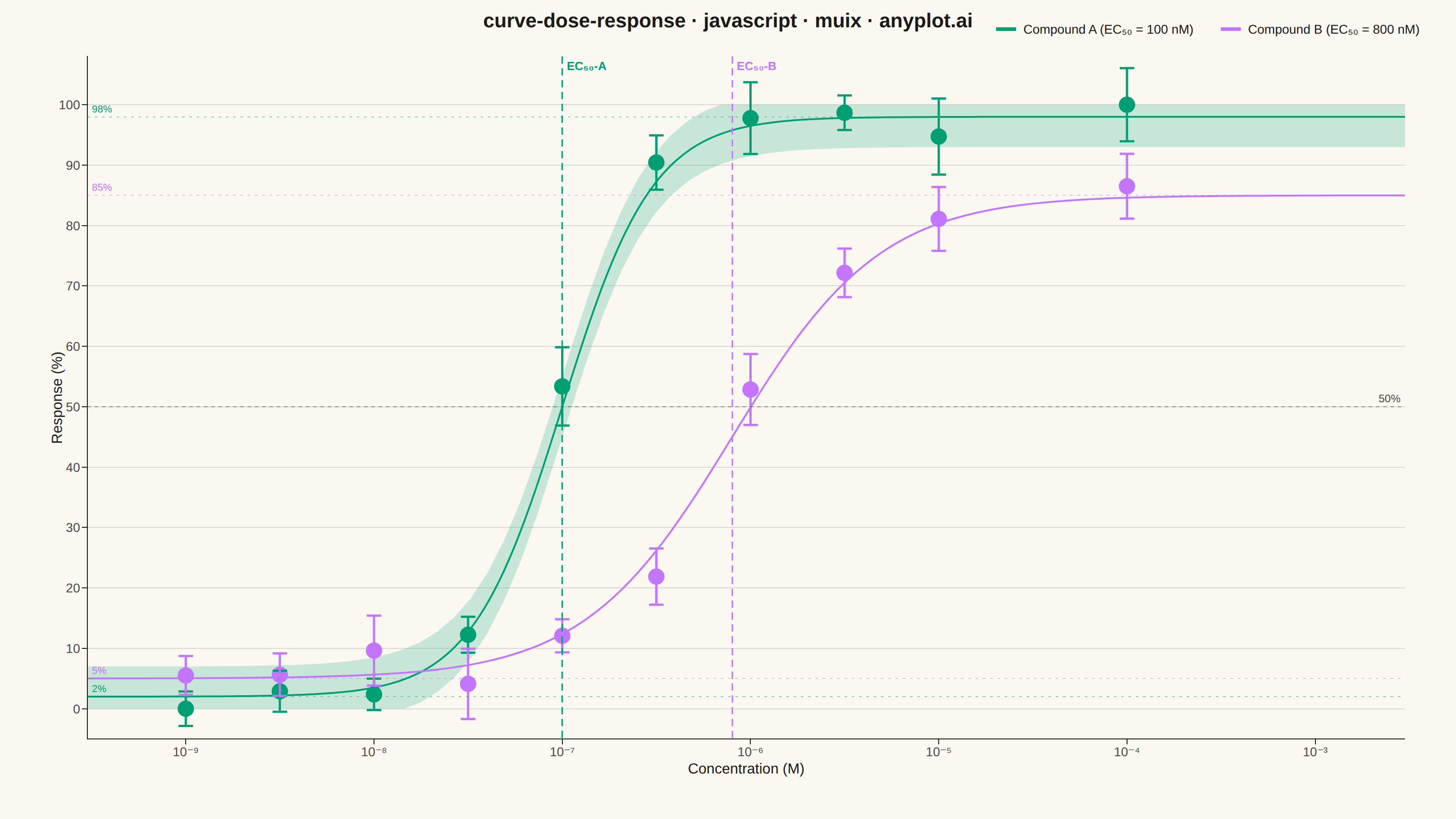
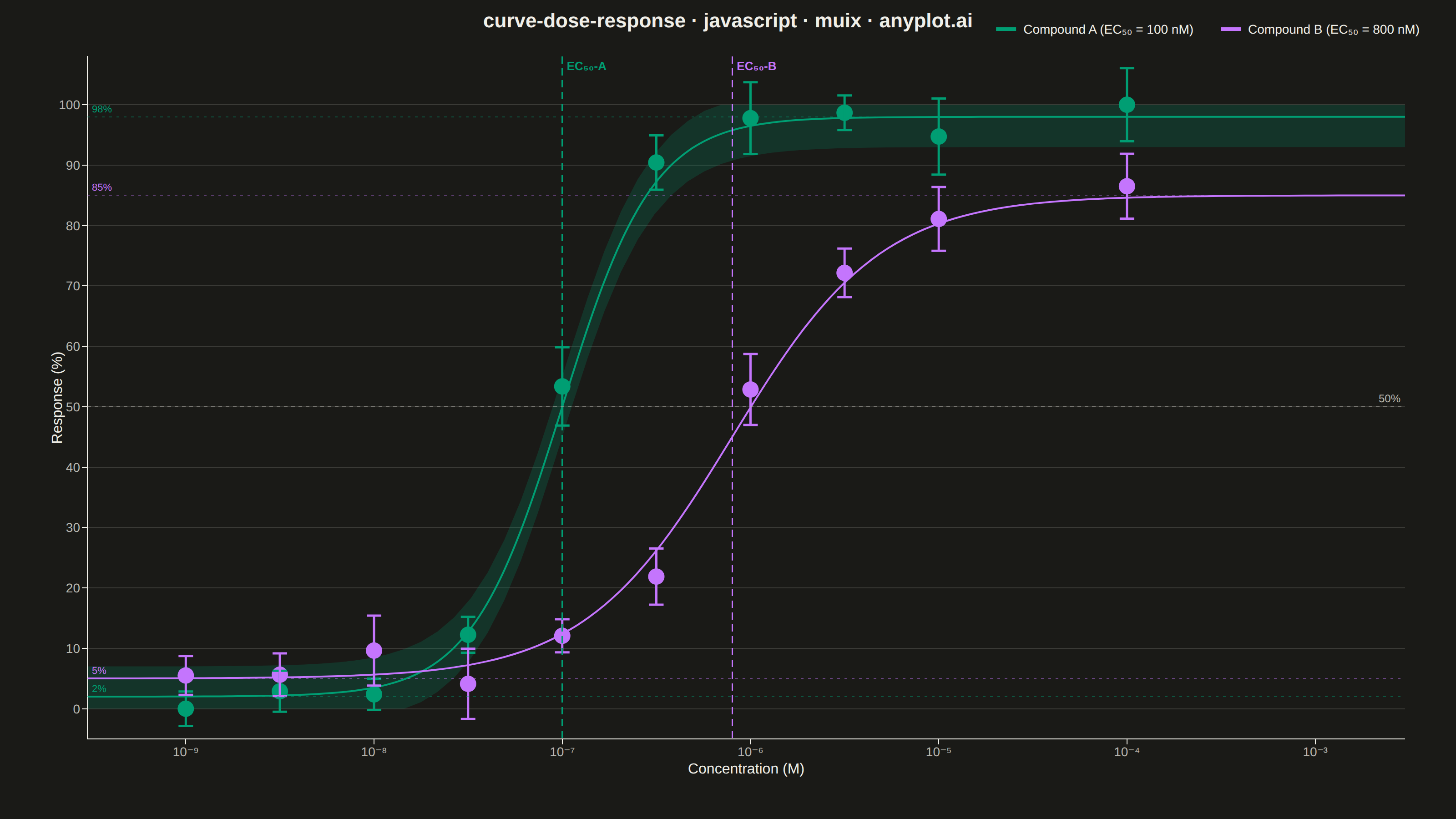
The same plot in 14 other libraries — JavaScript: Chart.js, D3.js, Apache ECharts, Highcharts; Python: Altair, Bokeh, lets-plot, Matplotlib, Plotly, plotnine, Pygal, Seaborn; R: ggplot2; Julia: Makie.jl. Compare all 15 side by side: Pharmacological Dose-Response Curve in Python, R, Julia and JavaScript.
A sigmoidal dose-response curve that plots biological response against drug concentration on a logarithmic x-axis, fitted using a four-parameter logistic (4PL) model. This visualization is essential for determining drug potency metrics such as EC50 (half-maximal effective concentration) or IC50 (half-maximal inhibitory concentration), Hill slope steepness, and upper/lower response asymptotes. It enables rapid visual comparison of compound efficacy and is a standard tool in pharmacological analysis.
// anyplot.ai
// curve-dose-response: Pharmacological Dose-Response Curve
// Library: muix 7.29.1 | JavaScript 22.22.3
// Quality: 89/100 | Created: 2026-06-24
//# anyplot-orientation: landscape
// anyplot.ai
// curve-dose-response: Pharmacological Dose-Response Curve
// Library: MUI X Charts | React | Node 22
// License: @mui/x-charts — MIT (community). Pro/Premium are out of scope.
// Quality: pending | Created: 2026-06-24

import { ChartContainer } from "@mui/x-charts/ChartContainer";
import { LinePlot } from "@mui/x-charts/LineChart";
import { ScatterPlot } from "@mui/x-charts/ScatterChart";
import { ChartsXAxis } from "@mui/x-charts/ChartsXAxis";
import { ChartsYAxis } from "@mui/x-charts/ChartsYAxis";
import { ChartsGrid } from "@mui/x-charts/ChartsGrid";
import { ChartsLegend } from "@mui/x-charts/ChartsLegend";
import { ChartsReferenceLine } from "@mui/x-charts/ChartsReferenceLine";
import { useXScale, useYScale } from "@mui/x-charts/hooks";

const t = window.ANYPLOT_TOKENS;
const { width, height } = window.ANYPLOT_SIZE;

// Four-parameter logistic model (4PL)
function fourPL(c, bottom, top, ec50, hill) {
  return bottom + (top - bottom) / (1 + Math.pow(ec50 / c, hill));
}

// Reproducible LCG (seed 42) — no Math.random() in browser harness context
let seed = 42;
function rng() {
  seed = (1664525 * seed + 1013904223) >>> 0;
  return seed / 4294967296;
}

// Unicode superscript formatter for log10 tick labels (e.g. 10⁻⁹)
const SUPERSCRIPT = { '0': '⁰', '1': '¹', '2': '²', '3': '³', '4': '⁴', '5': '⁵', '6': '⁶', '7': '⁷', '8': '⁸', '9': '⁹', '-': '⁻' };
function toSuperscript(n) {
  return String(n).split('').map(c => SUPERSCRIPT[c] || c).join('');
}

// Compound pharmacological parameters
const compA = { label: "Compound A (EC₅₀ = 100 nM)", bottom: 2, top: 98, ec50: 1e-7, hill: 1.8 };
const compB = { label: "Compound B (EC₅₀ = 800 nM)", bottom: 5, top: 85, ec50: 8e-7, hill: 1.1 };

// Ten measured concentrations per compound spanning 1 nM – 100 µM
const measConcs = [1e-9, 3.16e-9, 1e-8, 3.16e-8, 1e-7, 3.16e-7, 1e-6, 3.16e-6, 1e-5, 1e-4];

function makeMeasured(comp, idPrefix) {
  return measConcs.map((c, i) => ({
    x: c,
    y: Math.max(0, Math.min(100, fourPL(c, comp.bottom, comp.top, comp.ec50, comp.hill) + (rng() - 0.5) * 9)),
    sem: 2.5 + rng() * 4,
    id: `${idPrefix}-${i}`,
  }));
}

const measA = makeMeasured(compA, "A");
const measB = makeMeasured(compB, "B");

// Dense log-spaced x-axis for smooth fitted curves (80 points)
const N = 80;
const logMin = Math.log10(3e-10);
const logMax = Math.log10(3e-3);
const curveXs = Array.from({ length: N }, (_, i) =>
  Math.pow(10, logMin + (i / (N - 1)) * (logMax - logMin))
);

const curveAY = curveXs.map(x => fourPL(x, compA.bottom, compA.top, compA.ec50, compA.hill));
const curveBY = curveXs.map(x => fourPL(x, compB.bottom, compB.top, compB.ec50, compB.hill));

// 95% CI band for Compound A (±5 pp approximation)
const ciUpper = curveAY.map(y => Math.min(100, y + 5));
const ciLower = curveAY.map(y => Math.max(0, y - 5));

// Y-midpoint for the 50% response reference line
const midA = (compA.bottom + compA.top) / 2;

// Custom 95% CI band polygon rendered via MUI X axis scale hooks
function CIBand() {
  const xScale = useXScale();
  const yScale = useYScale();
  if (!xScale || !yScale) return null;

  const upper = curveXs.map((x, i) => [xScale(x), yScale(ciUpper[i])]);
  const lower = curveXs.map((x, i) => [xScale(x), yScale(ciLower[i])]);
  const pts = [...upper, ...lower.slice().reverse()];
  const d =
    pts.map((p, i) => `${i === 0 ? "M" : "L"}${p[0].toFixed(1)},${p[1].toFixed(1)}`).join(" ") + " Z";

  return <path d={d} fill={t.palette[0]} fillOpacity={0.20} stroke="none" />;
}

// SEM error bars rendered directly as SVG lines
function ErrorBars({ data, color }) {
  const xScale = useXScale();
  const yScale = useYScale();
  if (!xScale || !yScale) return null;

  const cap = 8;
  return (
    <g>
      {data.map(d => {
        const cx = xScale(d.x);
        const ytop = yScale(d.y + d.sem);
        const ybot = yScale(d.y - d.sem);
        if (isNaN(cx) || isNaN(ytop) || isNaN(ybot)) return null;
        return (
          <g key={d.id}>
            <line x1={cx} y1={ytop} x2={cx} y2={ybot} stroke={color} strokeWidth={2.5} />
            <line x1={cx - cap} y1={ytop} x2={cx + cap} y2={ytop} stroke={color} strokeWidth={2.5} />
            <line x1={cx - cap} y1={ybot} x2={cx + cap} y2={ybot} stroke={color} strokeWidth={2.5} />
          </g>
        );
      })}
    </g>
  );
}

const TITLE = "curve-dose-response · javascript · muix · anyplot.ai";

export default function Chart() {
  return (
    <ChartContainer
      width={width}
      height={height}
      margin={{ top: 62, right: 56, bottom: 88, left: 96 }}
      sx={{ '& .MuiChartsAxis-top, & .MuiChartsAxis-right': { display: 'none' } }}
      series={[
        {
          type: "line",
          id: "curveA",
          data: curveAY,
          label: compA.label,
          color: t.palette[0],
          showMark: false,
          curve: "monotoneX",
          xAxisId: "concentration",
        },
        {
          type: "line",
          id: "curveB",
          data: curveBY,
          label: compB.label,
          color: t.palette[1],
          showMark: false,
          curve: "monotoneX",
          xAxisId: "concentration",
        },
        {
          type: "scatter",
          id: "dataA",
          data: measA,
          color: t.palette[0],
          markerSize: 9,
          xAxisId: "concentration",
        },
        {
          type: "scatter",
          id: "dataB",
          data: measB,
          color: t.palette[1],
          markerSize: 9,
          xAxisId: "concentration",
        },
      ]}
      xAxis={[{
        id: "concentration",
        scaleType: "log",
        data: curveXs,
        min: 3e-10,
        max: 3e-3,
        label: "Concentration (M)",
        tickInterval: [1e-9, 1e-8, 1e-7, 1e-6, 1e-5, 1e-4, 1e-3],
        valueFormatter: v => `10${toSuperscript(Math.round(Math.log10(v)))}`,
        tickLabelStyle: { fontSize: 14, fill: t.inkSoft },
        labelStyle: { fontSize: 16, fill: t.ink },
      }]}
      yAxis={[{
        id: "response",
        min: -5,
        max: 108,
        label: "Response (%)",
        tickLabelStyle: { fontSize: 14, fill: t.inkSoft },
        labelStyle: { fontSize: 16, fill: t.ink },
      }]}
    >
      <ChartsGrid horizontal />
      <CIBand />
      <LinePlot skipAnimation />
      <ScatterPlot skipAnimation />
      <ErrorBars data={measA} color={t.palette[0]} />
      <ErrorBars data={measB} color={t.palette[1]} />
      <ChartsXAxis
        axisId="concentration"
        tickLabelStyle={{ fontSize: 14, fill: t.inkSoft }}
        labelStyle={{ fontSize: 16, fill: t.ink }}
      />
      <ChartsYAxis
        axisId="response"
        tickLabelStyle={{ fontSize: 14, fill: t.inkSoft }}
        labelStyle={{ fontSize: 16, fill: t.ink }}
      />
      <ChartsReferenceLine
        x={compA.ec50}
        axisId="concentration"
        label="EC₅₀-A"
        labelAlign="start"
        labelStyle={{ fill: t.palette[0], fontSize: 13, fontWeight: "bold" }}
        lineStyle={{ stroke: t.palette[0], strokeDasharray: "8,5", strokeWidth: 1.5 }}
      />
      <ChartsReferenceLine
        x={compB.ec50}
        axisId="concentration"
        label="EC₅₀-B"
        labelAlign="start"
        labelStyle={{ fill: t.palette[1], fontSize: 13, fontWeight: "bold" }}
        lineStyle={{ stroke: t.palette[1], strokeDasharray: "8,5", strokeWidth: 1.5 }}
      />
      <ChartsReferenceLine
        y={midA}
        axisId="response"
        label="50%"
        labelAlign="end"
        labelStyle={{ fill: t.inkSoft, fontSize: 12 }}
        lineStyle={{ stroke: t.inkSoft, strokeDasharray: "4,4", strokeWidth: 1, opacity: 0.55 }}
      />
      {/* Top asymptotes — Compound A (98%) and Compound B (85%) */}
      <ChartsReferenceLine
        y={compA.top}
        axisId="response"
        label={`${compA.top}%`}
        labelAlign="start"
        labelStyle={{ fill: t.palette[0], fontSize: 11 }}
        lineStyle={{ stroke: t.palette[0], strokeDasharray: "3,5", strokeWidth: 1, opacity: 0.45 }}
      />
      <ChartsReferenceLine
        y={compB.top}
        axisId="response"
        label={`${compB.top}%`}
        labelAlign="start"
        labelStyle={{ fill: t.palette[1], fontSize: 11 }}
        lineStyle={{ stroke: t.palette[1], strokeDasharray: "3,5", strokeWidth: 1, opacity: 0.45 }}
      />
      {/* Bottom asymptotes — Compound A (2%) and Compound B (5%) */}
      <ChartsReferenceLine
        y={compA.bottom}
        axisId="response"
        label={`${compA.bottom}%`}
        labelAlign="start"
        labelStyle={{ fill: t.palette[0], fontSize: 11 }}
        lineStyle={{ stroke: t.palette[0], strokeDasharray: "3,5", strokeWidth: 1, opacity: 0.45 }}
      />
      <ChartsReferenceLine
        y={compB.bottom}
        axisId="response"
        label={`${compB.bottom}%`}
        labelAlign="start"
        labelStyle={{ fill: t.palette[1], fontSize: 11 }}
        lineStyle={{ stroke: t.palette[1], strokeDasharray: "3,5", strokeWidth: 1, opacity: 0.45 }}
      />
      <ChartsLegend
        position={{ vertical: "top", horizontal: "right" }}
        slotProps={{
          legend: {
            itemMarkWidth: 22,
            itemMarkHeight: 4,
            markGap: 8,
            itemGap: 30,
            labelStyle: { fontSize: 14, fill: t.ink },
          },
        }}
      />
      <text
        x={width / 2}
        y={30}
        textAnchor="middle"
        fontSize={22}
        fontWeight={600}
        fill={t.ink}
      >
        {TITLE}
      </text>
    </ChartContainer>
  );
}
Runnable source as JSON, for any HTTP client: https://api.anyplot.ai/specs/curve-dose-response/muix/code. Any spec id and library id listed in llms-full.txt fit the same URL shape; every URL below is complete and callable.
{
  "spec_id": "curve-dose-response",
  "language": "javascript",
  "library": "muix",
  "page": "https://anyplot.ai/curve-dose-response/javascript/muix",
  "hub": "https://anyplot.ai/curve-dose-response",
  "code_json": "https://api.anyplot.ai/specs/curve-dose-response/muix/code",
  "spec_json": "https://api.anyplot.ai/specs/curve-dose-response",
  "render_light_png": "https://storage.googleapis.com/anyplot-images/plots/curve-dose-response/javascript/muix/plot-light.png",
  "render_dark_png": "https://storage.googleapis.com/anyplot-images/plots/curve-dose-response/javascript/muix/plot-dark.png",
  "interactive_light_html": "https://storage.googleapis.com/anyplot-images/plots/curve-dose-response/javascript/muix/plot-light.html",
  "interactive_dark_html": "https://storage.googleapis.com/anyplot-images/plots/curve-dose-response/javascript/muix/plot-dark.html",
  "quality_score": 89.0,
  "license": "MIT",
  "guide": "https://anyplot.ai/llms.txt"
}
Part of Pharmacological Dose-Response Curve on anyplot.ai.