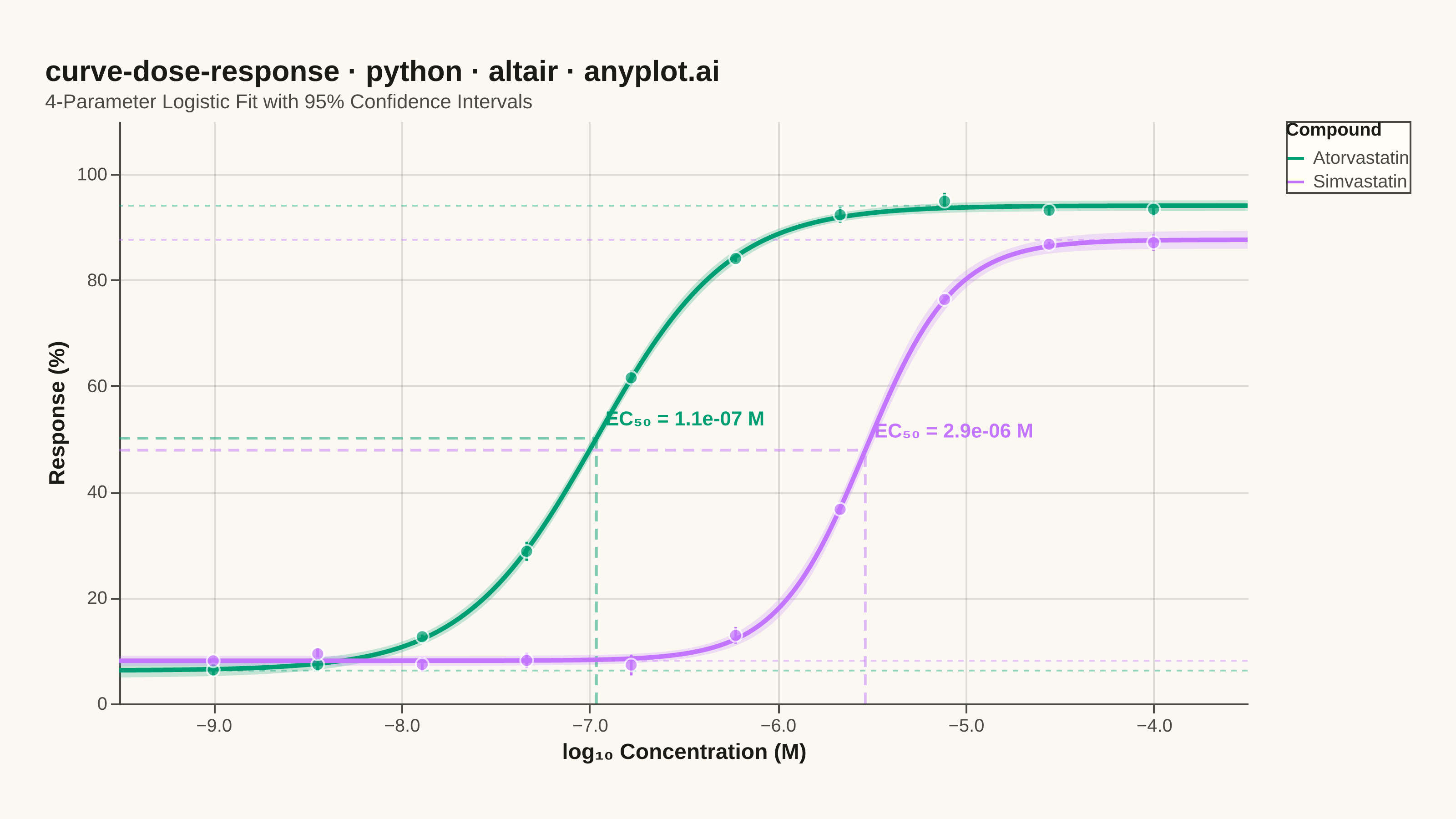
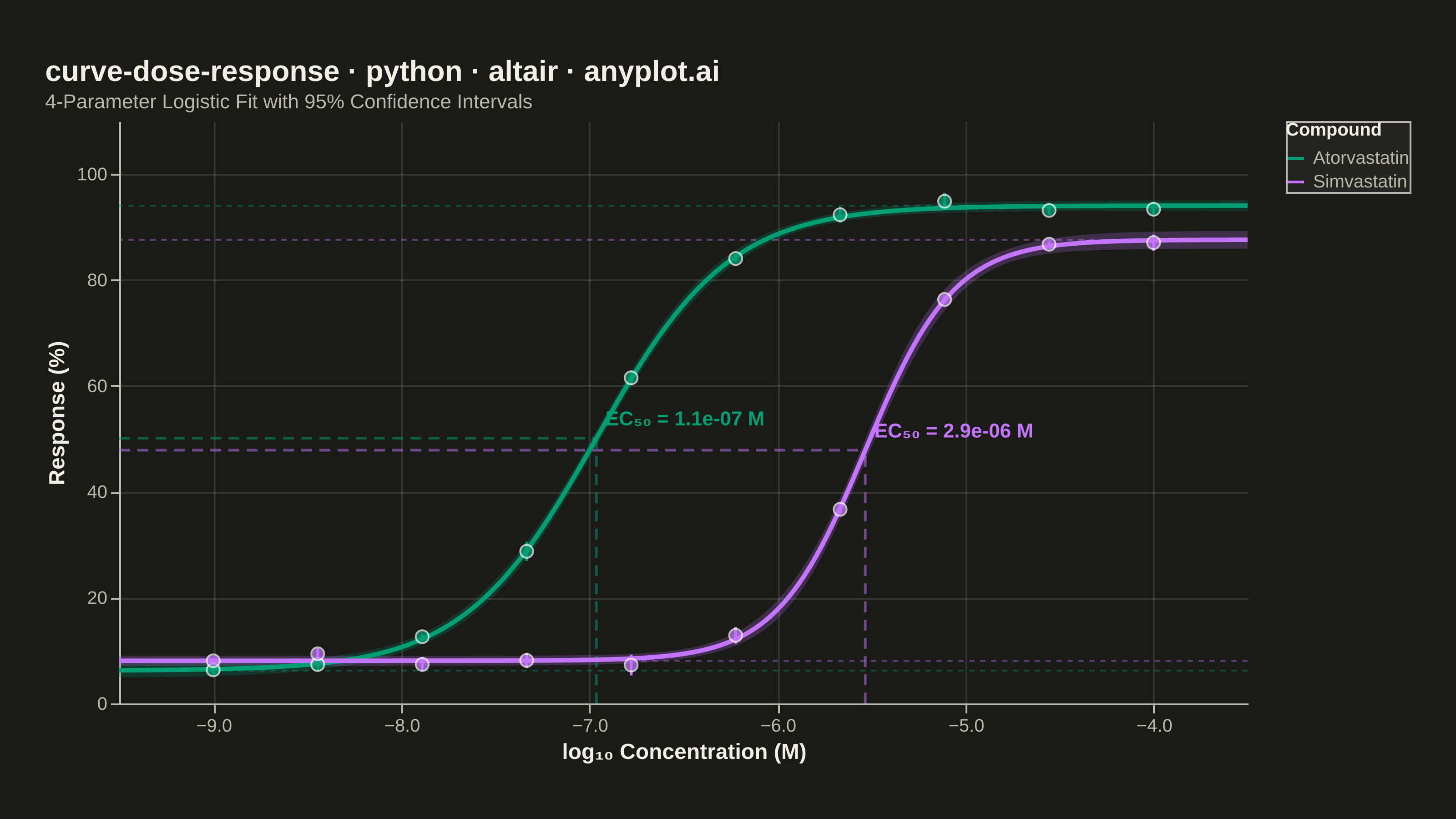
A sigmoidal dose-response curve that plots biological response against drug concentration on a logarithmic x-axis, fitted using a four-parameter logistic (4PL) model. This visualization is essential for determining drug potency metrics such as EC50 (half-maximal effective concentration) or IC50 (half-maximal inhibitory concentration), Hill slope steepness, and upper/lower response asymptotes. It enables rapid visual comparison of compound efficacy and is a standard tool in pharmacological analysis.
""" anyplot.ai
curve-dose-response: Pharmacological Dose-Response Curve
Library: altair 6.2.2 | Python 3.13.14
Quality: 91/100 | Updated: 2026-06-24
"""

import os

import altair as alt
import numpy as np
import pandas as pd
from PIL import Image
from scipy.optimize import curve_fit
from scipy.stats import t as t_dist


# Theme-adaptive chrome tokens (Imprint palette)
THEME = os.getenv("ANYPLOT_THEME", "light")
PAGE_BG = "#FAF8F1" if THEME == "light" else "#1A1A17"
ELEVATED_BG = "#FFFDF6" if THEME == "light" else "#242420"
INK = "#1A1A17" if THEME == "light" else "#F0EFE8"
INK_SOFT = "#4A4A44" if THEME == "light" else "#B8B7B0"
INK_MUTED = "#6B6A63" if THEME == "light" else "#A8A79F"

# Imprint palette — positions 1 and 2 for two-series categorical
IMPRINT_PALETTE = ["#009E73", "#C475FD", "#4467A3", "#BD8233", "#AE3030", "#2ABCCD", "#954477", "#99B314"]

# Data
np.random.seed(42)
concentrations = np.logspace(-9, -4, 10)


def logistic_4pl(x, bottom, top, ec50, hill):
    return bottom + (top - bottom) / (1 + (ec50 / x) ** hill)


compound_params = {
    "Atorvastatin": {"bottom": 5, "top": 95, "ec50": 1e-7, "hill": 1.2},
    "Simvastatin": {"bottom": 8, "top": 88, "ec50": 3e-6, "hill": 1.8},
}

rows = []
for name, params in compound_params.items():
    true_response = logistic_4pl(concentrations, params["bottom"], params["top"], params["ec50"], params["hill"])
    noise = np.random.normal(0, 3, size=(5, len(concentrations)))
    replicates = true_response + noise
    means = replicates.mean(axis=0)
    sems = replicates.std(axis=0, ddof=1) / np.sqrt(5)
    for c, m, s in zip(concentrations, means, sems, strict=True):
        rows.append(
            {
                "concentration": c,
                "log_conc": np.log10(c),
                "response": m,
                "sem": s,
                "response_upper": m + s,
                "response_lower": m - s,
                "compound": name,
            }
        )

df = pd.DataFrame(rows)

# Fit 4PL curves, compute smooth fit lines and 95% CI via delta method
fit_rows = []
ref_rows = []
ci_rows = []

for name, group in df.groupby("compound"):
    xdata = group["concentration"].values
    ydata = group["response"].values
    params_init = compound_params[name]
    p0 = [params_init["bottom"], params_init["top"], params_init["ec50"], params_init["hill"]]

    popt, pcov = curve_fit(logistic_4pl, xdata, ydata, p0=p0, maxfev=10000)
    bottom_fit, top_fit, ec50_fit, hill_fit = popt

    x_smooth = np.logspace(-9.5, -3.5, 200)
    y_smooth = logistic_4pl(x_smooth, *popt)
    for xs, ys in zip(x_smooth, y_smooth, strict=True):
        fit_rows.append({"log_conc": np.log10(xs), "response": ys, "compound": name})

    n = len(xdata)
    dof = n - len(popt)
    t_val = t_dist.ppf(0.975, dof)

    jacobian = np.zeros((len(x_smooth), 4))
    for i, xs in enumerate(x_smooth):
        ratio = (ec50_fit / xs) ** hill_fit
        denom = 1 + ratio
        jacobian[i, 0] = 1 - 1 / denom
        jacobian[i, 1] = 1 / denom
        jacobian[i, 2] = -(top_fit - bottom_fit) * hill_fit * ratio / (ec50_fit * denom**2)
        jacobian[i, 3] = -(top_fit - bottom_fit) * ratio * np.log(ec50_fit / xs) / denom**2

    pred_var = np.array([j @ pcov @ j for j in jacobian])
    pred_se = np.sqrt(np.maximum(pred_var, 0))
    ci_upper = logistic_4pl(x_smooth, *popt) + t_val * pred_se
    ci_lower = logistic_4pl(x_smooth, *popt) - t_val * pred_se
    for xs, cu, cl in zip(x_smooth, ci_upper, ci_lower, strict=True):
        ci_rows.append({"log_conc": np.log10(xs), "ci_upper": cu, "ci_lower": cl, "compound": name})

    half_response = (bottom_fit + top_fit) / 2
    ec50_sci = f"{ec50_fit:.1e}"
    ref_rows.append(
        {
            "compound": name,
            "ec50_log": np.log10(ec50_fit),
            "half_response": half_response,
            "bottom_fit": bottom_fit,
            "top_fit": top_fit,
            "ec50_label": f"EC₅₀ = {ec50_sci} M",
            "x_left": -9.5,  # left edge of x-domain for clipped hline
            "y_bottom": 0.0,  # bottom of y-domain for clipped vline
        }
    )

df_fit = pd.DataFrame(fit_rows)
df_ci = pd.DataFrame(ci_rows)
df_ref = pd.DataFrame(ref_rows)

# Color scale — Imprint positions 1 (#009E73) and 2 (#C475FD)
color_scale = alt.Scale(domain=["Atorvastatin", "Simvastatin"], range=[IMPRINT_PALETTE[0], IMPRINT_PALETTE[1]])
# Shared encoding shortcuts for multi-layer color consistency
color_no_legend = alt.Color("compound:N", scale=color_scale, legend=None)
color_with_legend = alt.Color("compound:N", scale=color_scale, legend=alt.Legend(title="Compound"))

# Nearest-point hover selection
nearest = alt.selection_point(nearest=True, on="pointerover", fields=["log_conc"], empty=False)

base_x = alt.X(
    "log_conc:Q",
    title="log₁₀ Concentration (M)",
    scale=alt.Scale(domain=[-9.5, -3.5]),
    axis=alt.Axis(values=list(range(-9, -3))),
)
base_y = alt.Y(
    "response:Q", title="Response (%)", scale=alt.Scale(domain=[0, 105]), axis=alt.Axis(values=[0, 20, 40, 60, 80, 100])
)

# 95% CI shaded bands
ci_band = (
    alt.Chart(df_ci)
    .mark_area(opacity=0.22)
    .encode(x=alt.X("log_conc:Q"), y=alt.Y("ci_lower:Q"), y2="ci_upper:Q", color=color_no_legend)
)

# Fitted 4PL curves — legend anchor layer
fitted_lines = (
    alt.Chart(df_fit).mark_line(strokeWidth=2.5).encode(x=alt.X("log_conc:Q"), y=base_y, color=color_with_legend)
)

# SEM error bars
error_bars = (
    alt.Chart(df)
    .mark_rule(strokeWidth=1.5)
    .encode(x=alt.X("log_conc:Q"), y=alt.Y("response_lower:Q"), y2="response_upper:Q", color=color_no_legend)
)

# Invisible hover capture layer
select_layer = (
    alt.Chart(df)
    .mark_point(size=200, opacity=0)
    .encode(x=alt.X("log_conc:Q"), y=alt.Y("response:Q"))
    .add_params(nearest)
)

# Hover crosshair
hover_rule = (
    alt.Chart(df)
    .mark_rule(strokeWidth=1, color=INK_MUTED, strokeDash=[3, 3])
    .encode(x=alt.X("log_conc:Q"))
    .transform_filter(nearest)
)

# Data points with hover-size interaction and tooltips
data_points = (
    alt.Chart(df)
    .mark_point(filled=True, stroke="white", strokeWidth=1)
    .encode(
        x=base_x,
        y=base_y,
        color=color_no_legend,
        size=alt.condition(nearest, alt.value(100), alt.value(50)),
        tooltip=[
            alt.Tooltip("compound:N", title="Compound"),
            alt.Tooltip("log_conc:Q", title="log₁₀ [C]", format=".2f"),
            alt.Tooltip("response:Q", title="Response (%)", format=".1f"),
            alt.Tooltip("sem:Q", title="SEM", format=".2f"),
        ],
    )
)

# EC50 reference lines — clipped to form an "L" pointing at the EC50 intersection.
# Horizontal: left edge → EC50 x-position (avoids cluttering the right half)
ec50_hlines = (
    alt.Chart(df_ref)
    .mark_rule(strokeDash=[6, 4], strokeWidth=1.5, opacity=0.5)
    .encode(x=alt.X("x_left:Q"), x2="ec50_log:Q", y=alt.Y("half_response:Q"), color=color_no_legend)
)

# Vertical: bottom → half-response (drops down to the x-axis)
ec50_vlines = (
    alt.Chart(df_ref)
    .mark_rule(strokeDash=[6, 4], strokeWidth=1.5, opacity=0.5)
    .encode(x=alt.X("ec50_log:Q"), y=alt.Y("y_bottom:Q"), y2="half_response:Q", color=color_no_legend)
)

# Top and bottom asymptote guides
asymptote_top = (
    alt.Chart(df_ref)
    .mark_rule(strokeDash=[3, 3], strokeWidth=1, opacity=0.4)
    .encode(y=alt.Y("top_fit:Q"), color=color_no_legend)
)

asymptote_bottom = (
    alt.Chart(df_ref)
    .mark_rule(strokeDash=[3, 3], strokeWidth=1, opacity=0.4)
    .encode(y=alt.Y("bottom_fit:Q"), color=color_no_legend)
)

# EC50 value labels — offset above the intersection to avoid overlap with reference lines
ec50_labels = (
    alt.Chart(df_ref)
    .mark_text(fontSize=11, fontWeight="bold", align="left", dx=5, dy=-10)
    .encode(x=alt.X("ec50_log:Q"), y=alt.Y("half_response:Q"), text=alt.Text("ec50_label:N"), color=color_no_legend)
)

# Compose — resolve_scale(color="independent") needed because layers span
# four distinct DataFrames (df, df_fit, df_ci, df_ref); each layer's explicit
# scale range is identical, so colors stay consistent across layers.
chart = (
    (
        ci_band
        + asymptote_top
        + asymptote_bottom
        + ec50_hlines
        + ec50_vlines
        + fitted_lines
        + error_bars
        + data_points
        + ec50_labels
        + select_layer
        + hover_rule
    )
    .resolve_scale(color="independent")
    .properties(
        width=620,
        height=320,
        background=PAGE_BG,
        title=alt.Title(
            "curve-dose-response · python · altair · anyplot.ai",
            subtitle="4-Parameter Logistic Fit with 95% Confidence Intervals",
            fontSize=16,
            subtitleFontSize=11,
            subtitleColor=INK_SOFT,
            color=INK,
            anchor="start",
        ),
    )
    .configure_view(fill=PAGE_BG, strokeWidth=0)
    .configure_title(color=INK)
    .configure_axis(
        labelFontSize=10,
        titleFontSize=12,
        labelColor=INK_SOFT,
        titleColor=INK,
        gridColor=INK,
        gridOpacity=0.12,
        domainColor=INK_SOFT,
        tickColor=INK_SOFT,
    )
    .configure_legend(
        titleFontSize=10,
        labelFontSize=10,
        symbolSize=80,
        labelColor=INK_SOFT,
        titleColor=INK,
        fillColor=ELEVATED_BG,
        strokeColor=INK_SOFT,
    )
)

# Save — scale_factor=4.0 with width=620, height=320 targets 3200×1800
TW, TH = 3200, 1800
chart.save(f"plot-{THEME}.png", scale_factor=4.0)
chart.save(f"plot-{THEME}.html")

# Pad PNG to exact target (vl-convert can land slightly short; never crop)
_img = Image.open(f"plot-{THEME}.png").convert("RGB")
_w, _h = _img.size
if _w > TW or _h > TH:
    raise SystemExit(
        f"altair vl-convert produced {_w}×{_h}, exceeds target {TW}×{TH}. "
        f"Shrink chart .properties(width=, height=) values and re-render."
    )
if _w < TW or _h < TH:
    _canvas = Image.new("RGB", (TW, TH), PAGE_BG)
    _canvas.paste(_img, ((TW - _w) // 2, (TH - _h) // 2))
    _canvas.save(f"plot-{THEME}.png")
Runnable source as JSON, for any HTTP client: https://api.anyplot.ai/specs/curve-dose-response/altair/code. Any spec id and library id listed in llms-full.txt fit the same URL shape; every URL below is complete and callable.
{
  "spec_id": "curve-dose-response",
  "language": "python",
  "library": "altair",
  "page": "https://anyplot.ai/curve-dose-response/python/altair",
  "hub": "https://anyplot.ai/curve-dose-response",
  "code_json": "https://api.anyplot.ai/specs/curve-dose-response/altair/code",
  "spec_json": "https://api.anyplot.ai/specs/curve-dose-response",
  "render_light_png": "https://storage.googleapis.com/anyplot-images/plots/curve-dose-response/python/altair/plot-light.png",
  "render_dark_png": "https://storage.googleapis.com/anyplot-images/plots/curve-dose-response/python/altair/plot-dark.png",
  "interactive_light_html": "https://storage.googleapis.com/anyplot-images/plots/curve-dose-response/python/altair/plot-light.html",
  "interactive_dark_html": "https://storage.googleapis.com/anyplot-images/plots/curve-dose-response/python/altair/plot-dark.html",
  "quality_score": 91.0,
  "license": "MIT",
  "guide": "https://anyplot.ai/llms.txt"
}
Part of Pharmacological Dose-Response Curve on anyplot.ai.