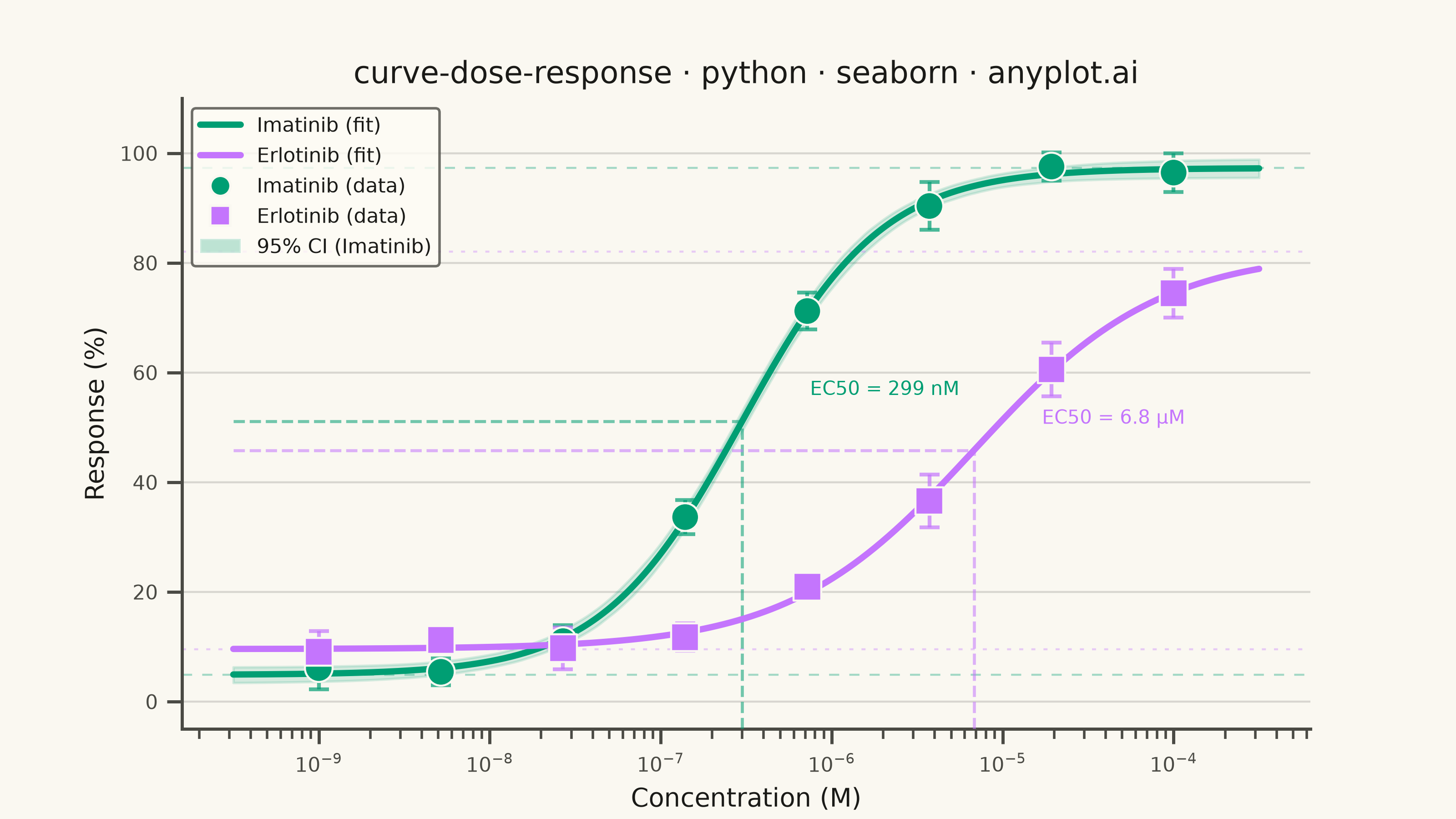
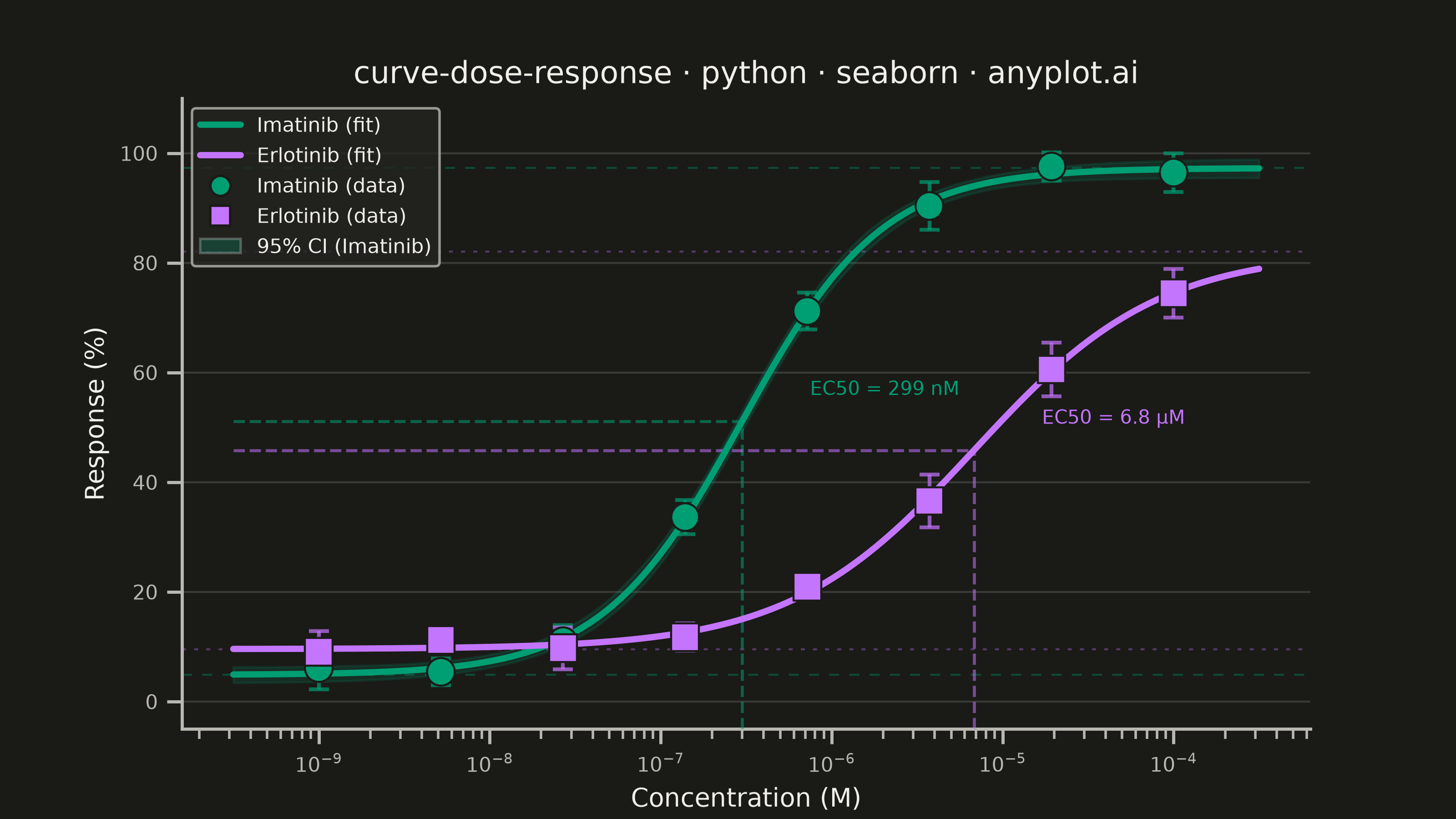
A sigmoidal dose-response curve that plots biological response against drug concentration on a logarithmic x-axis, fitted using a four-parameter logistic (4PL) model. This visualization is essential for determining drug potency metrics such as EC50 (half-maximal effective concentration) or IC50 (half-maximal inhibitory concentration), Hill slope steepness, and upper/lower response asymptotes. It enables rapid visual comparison of compound efficacy and is a standard tool in pharmacological analysis.
""" anyplot.ai
curve-dose-response: Pharmacological Dose-Response Curve
Library: seaborn 0.13.2 | Python 3.13.14
Quality: 93/100 | Updated: 2026-06-24
"""

import os

import matplotlib.pyplot as plt
import numpy as np
import pandas as pd
import seaborn as sns
from matplotlib.lines import Line2D
from matplotlib.patches import Patch
from scipy.optimize import curve_fit


# Theme tokens — Imprint palette (see prompts/default-style-guide.md)
THEME = os.getenv("ANYPLOT_THEME", "light")
PAGE_BG = "#FAF8F1" if THEME == "light" else "#1A1A17"
ELEVATED_BG = "#FFFDF6" if THEME == "light" else "#242420"
INK = "#1A1A17" if THEME == "light" else "#F0EFE8"
INK_SOFT = "#4A4A44" if THEME == "light" else "#B8B7B0"

IMPRINT_PALETTE = ["#009E73", "#C475FD", "#4467A3", "#BD8233", "#AE3030", "#2ABCCD", "#954477", "#99B314"]
COLOR_A = IMPRINT_PALETTE[0]  # brand green — Imatinib (first series, always #009E73)
COLOR_B = IMPRINT_PALETTE[1]  # lavender — Erlotinib
palette_dict = {"Imatinib": COLOR_A, "Erlotinib": COLOR_B}

sns.set_theme(
    style="ticks",
    rc={
        "figure.facecolor": PAGE_BG,
        "axes.facecolor": PAGE_BG,
        "axes.edgecolor": INK_SOFT,
        "axes.labelcolor": INK,
        "text.color": INK,
        "xtick.color": INK_SOFT,
        "ytick.color": INK_SOFT,
        "grid.color": INK,
        "grid.alpha": 0.15,
        "legend.facecolor": ELEVATED_BG,
        "legend.edgecolor": INK_SOFT,
    },
)

# Data — synthetic pharmacological dose-response for two kinase inhibitors
np.random.seed(42)

concentrations = np.logspace(-9, -4, 8)

bottom_a, top_a, ec50_a, hill_a = 5.0, 95.0, 3e-7, 1.2
bottom_b, top_b, ec50_b, hill_b = 10.0, 80.0, 5e-6, 0.9

# 4PL logistic: response = bottom + (top - bottom) / (1 + (ec50/conc)^hill)
logistic4pl = lambda conc, bottom, top, ec50, hill: bottom + (top - bottom) / (1 + (ec50 / conc) ** hill)

response_a = logistic4pl(concentrations, bottom_a, top_a, ec50_a, hill_a) + np.random.normal(0, 2, len(concentrations))
response_b = logistic4pl(concentrations, bottom_b, top_b, ec50_b, hill_b) + np.random.normal(0, 2, len(concentrations))
sem_a = np.random.uniform(2, 5, len(concentrations))
sem_b = np.random.uniform(2, 5, len(concentrations))

df = pd.concat(
    [
        pd.DataFrame({"concentration": concentrations, "response": response_a, "sem": sem_a, "compound": "Imatinib"}),
        pd.DataFrame({"concentration": concentrations, "response": response_b, "sem": sem_b, "compound": "Erlotinib"}),
    ],
    ignore_index=True,
)

# Fit 4PL models via scipy curve_fit
fit_params = {}
fit_cov = {}
for compound, p0 in [("Imatinib", [5, 95, 3e-7, 1.2]), ("Erlotinib", [10, 80, 5e-6, 0.9])]:
    mask = df["compound"] == compound
    popt, pcov = curve_fit(
        logistic4pl, df.loc[mask, "concentration"].values, df.loc[mask, "response"].values, p0=p0, maxfev=10000
    )
    fit_params[compound] = popt
    fit_cov[compound] = pcov

x_fit = np.logspace(-9.5, -3.5, 300)

# Parametric bootstrap 95% CI for Imatinib
n_boot = 300
param_samples = np.random.multivariate_normal(fit_params["Imatinib"], fit_cov["Imatinib"], size=n_boot)
boot_curves = np.array([logistic4pl(x_fit, *s) for s in param_samples])
ci_lo = np.percentile(boot_curves, 2.5, axis=0)
ci_hi = np.percentile(boot_curves, 97.5, axis=0)

# Long-format DataFrame for fitted curves (enables sns.lineplot hue+style mapping)
df_fit = pd.concat(
    [
        pd.DataFrame(
            {"concentration": x_fit, "response": logistic4pl(x_fit, *fit_params["Imatinib"]), "compound": "Imatinib"}
        ),
        pd.DataFrame(
            {"concentration": x_fit, "response": logistic4pl(x_fit, *fit_params["Erlotinib"]), "compound": "Erlotinib"}
        ),
    ],
    ignore_index=True,
)

# Plot — landscape 3200×1800 px (figsize=(8, 4.5) × dpi=400, no bbox_inches='tight')
fig, ax = plt.subplots(figsize=(8, 4.5), dpi=400, facecolor=PAGE_BG)
ax.set_facecolor(PAGE_BG)

# CI band — Imatinib only (spec: at least one fitted curve)
ax.fill_between(x_fit, ci_lo, ci_hi, color=COLOR_A, alpha=0.15, zorder=1)

# Fitted curves via sns.lineplot (idiomatic seaborn: hue+style over long-format DataFrame)
sns.lineplot(
    data=df_fit,
    x="concentration",
    y="response",
    hue="compound",
    hue_order=["Imatinib", "Erlotinib"],
    style="compound",
    dashes=False,
    palette=palette_dict,
    linewidth=2.5,
    zorder=4,
    ax=ax,
    legend=False,
)

# Data points (seaborn scatterplot for idiomatic hue+style mapping)
sns.scatterplot(
    data=df,
    x="concentration",
    y="response",
    hue="compound",
    style="compound",
    markers={"Imatinib": "o", "Erlotinib": "s"},
    palette=palette_dict,
    s=120,
    edgecolor=PAGE_BG,
    linewidth=0.8,
    zorder=5,
    ax=ax,
    legend=False,
)

# Error bars (seaborn scatterplot doesn't support yerr natively)
for compound in ["Imatinib", "Erlotinib"]:
    sub = df[df["compound"] == compound]
    ax.errorbar(
        sub["concentration"],
        sub["response"],
        yerr=sub["sem"],
        fmt="none",
        ecolor=palette_dict[compound],
        capsize=4,
        capthick=1.5,
        elinewidth=1.5,
        alpha=0.7,
        zorder=4,
    )

# EC50 dashed reference lines
for compound in ["Imatinib", "Erlotinib"]:
    popt = fit_params[compound]
    ec50_val = popt[2]
    half_resp = popt[0] + (popt[1] - popt[0]) / 2
    ax.hlines(
        half_resp,
        x_fit[0],
        ec50_val,
        colors=palette_dict[compound],
        linestyles="dashed",
        linewidth=1.2,
        alpha=0.55,
        zorder=3,
    )
    ax.vlines(
        ec50_val, -5, half_resp, colors=palette_dict[compound], linestyles="dashed", linewidth=1.2, alpha=0.55, zorder=3
    )

# EC50 value annotations near crosshair intersections
for compound in ["Imatinib", "Erlotinib"]:
    popt = fit_params[compound]
    ec50_val = popt[2]
    half_resp = popt[0] + (popt[1] - popt[0]) / 2
    if ec50_val < 1e-6:
        ec50_label = f"EC50 = {ec50_val * 1e9:.0f} nM"
    else:
        ec50_label = f"EC50 = {ec50_val * 1e6:.1f} μM"
    ax.text(
        ec50_val * 2.5, half_resp + 4, ec50_label, fontsize=7.5, color=palette_dict[compound], va="bottom", ha="left"
    )

# Asymptote reference lines (top and bottom plateaus)
for compound, dash in [("Imatinib", (5, 5)), ("Erlotinib", (2, 4))]:
    popt = fit_params[compound]
    ax.axhline(popt[0], color=palette_dict[compound], linestyle=(0, dash), linewidth=0.8, alpha=0.35, zorder=1)
    ax.axhline(popt[1], color=palette_dict[compound], linestyle=(0, dash), linewidth=0.8, alpha=0.35, zorder=1)

# Style
ax.set_xscale("log")
ax.set_xlabel("Concentration (M)", fontsize=10, color=INK)
ax.set_ylabel("Response (%)", fontsize=10, color=INK)
ax.set_title("curve-dose-response · python · seaborn · anyplot.ai", fontsize=12, fontweight="medium", color=INK)
ax.tick_params(axis="both", labelsize=8, colors=INK_SOFT)
sns.despine(ax=ax)
ax.yaxis.grid(True, alpha=0.15, linewidth=0.8)
ax.set_ylim(-5, 110)

# Custom legend (explicit handles for line + marker + CI patch)
legend_handles = [
    Line2D([0], [0], color=COLOR_A, linewidth=2.5, label="Imatinib (fit)"),
    Line2D([0], [0], color=COLOR_B, linewidth=2.5, label="Erlotinib (fit)"),
    Line2D(
        [0],
        [0],
        marker="o",
        color="none",
        markerfacecolor=COLOR_A,
        markersize=8,
        markeredgecolor=PAGE_BG,
        label="Imatinib (data)",
    ),
    Line2D(
        [0],
        [0],
        marker="s",
        color="none",
        markerfacecolor=COLOR_B,
        markersize=8,
        markeredgecolor=PAGE_BG,
        label="Erlotinib (data)",
    ),
    Patch(facecolor=COLOR_A, alpha=0.25, label="95% CI (Imatinib)"),
]
ax.legend(handles=legend_handles, fontsize=8, frameon=True, loc="upper left", facecolor=ELEVATED_BG, edgecolor=INK_SOFT)

# Save — bbox_inches omitted (must stay default None per seaborn canvas contract)
plt.savefig(f"plot-{THEME}.png", dpi=400, facecolor=PAGE_BG)
Runnable source as JSON, for any HTTP client: https://api.anyplot.ai/specs/curve-dose-response/seaborn/code. Any spec id and library id listed in llms-full.txt fit the same URL shape; every URL below is complete and callable.
{
  "spec_id": "curve-dose-response",
  "language": "python",
  "library": "seaborn",
  "page": "https://anyplot.ai/curve-dose-response/python/seaborn",
  "hub": "https://anyplot.ai/curve-dose-response",
  "code_json": "https://api.anyplot.ai/specs/curve-dose-response/seaborn/code",
  "spec_json": "https://api.anyplot.ai/specs/curve-dose-response",
  "render_light_png": "https://storage.googleapis.com/anyplot-images/plots/curve-dose-response/python/seaborn/plot-light.png",
  "render_dark_png": "https://storage.googleapis.com/anyplot-images/plots/curve-dose-response/python/seaborn/plot-dark.png",
  "quality_score": 93.0,
  "license": "MIT",
  "guide": "https://anyplot.ai/llms.txt"
}
Part of Pharmacological Dose-Response Curve on anyplot.ai.