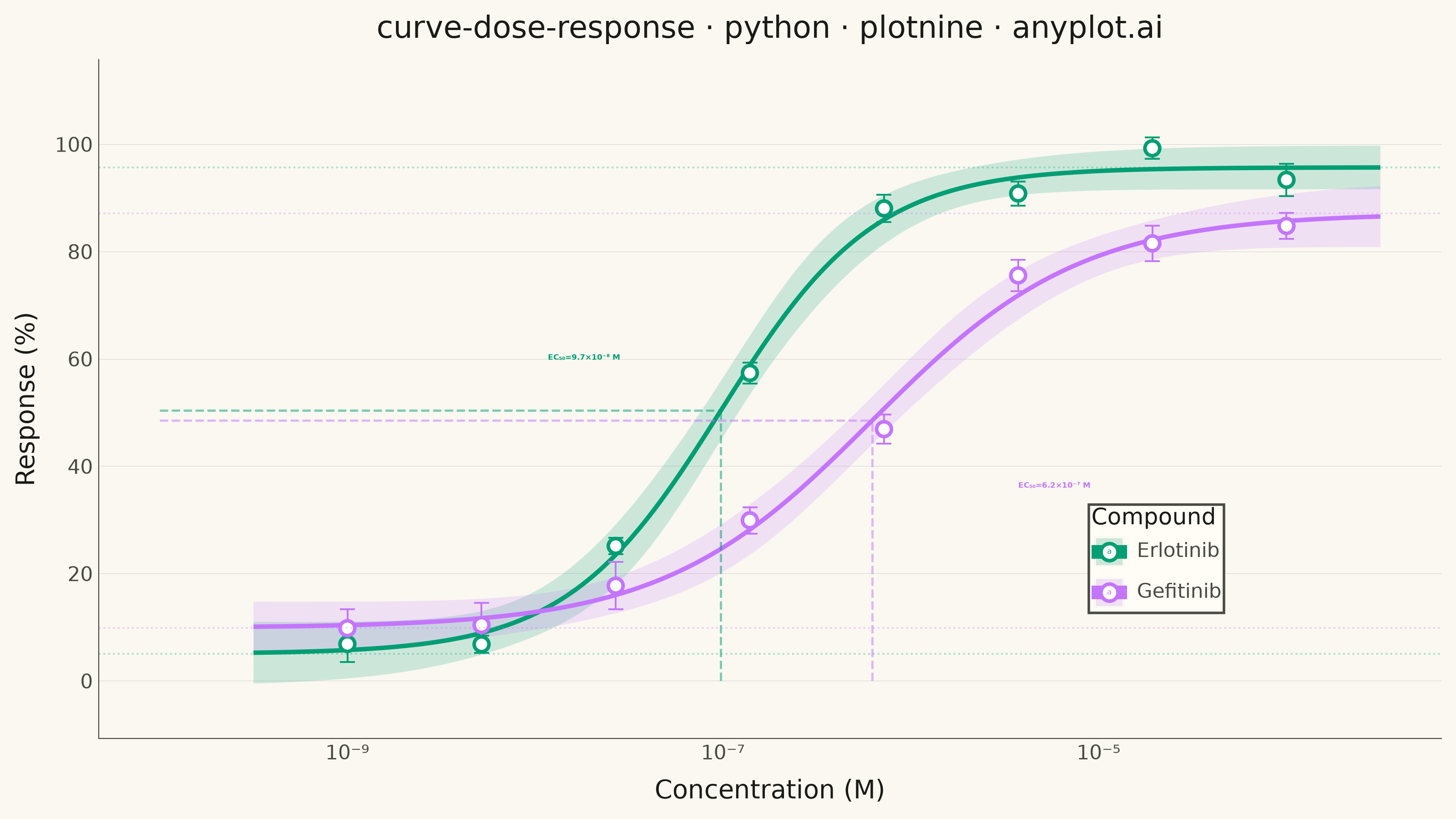
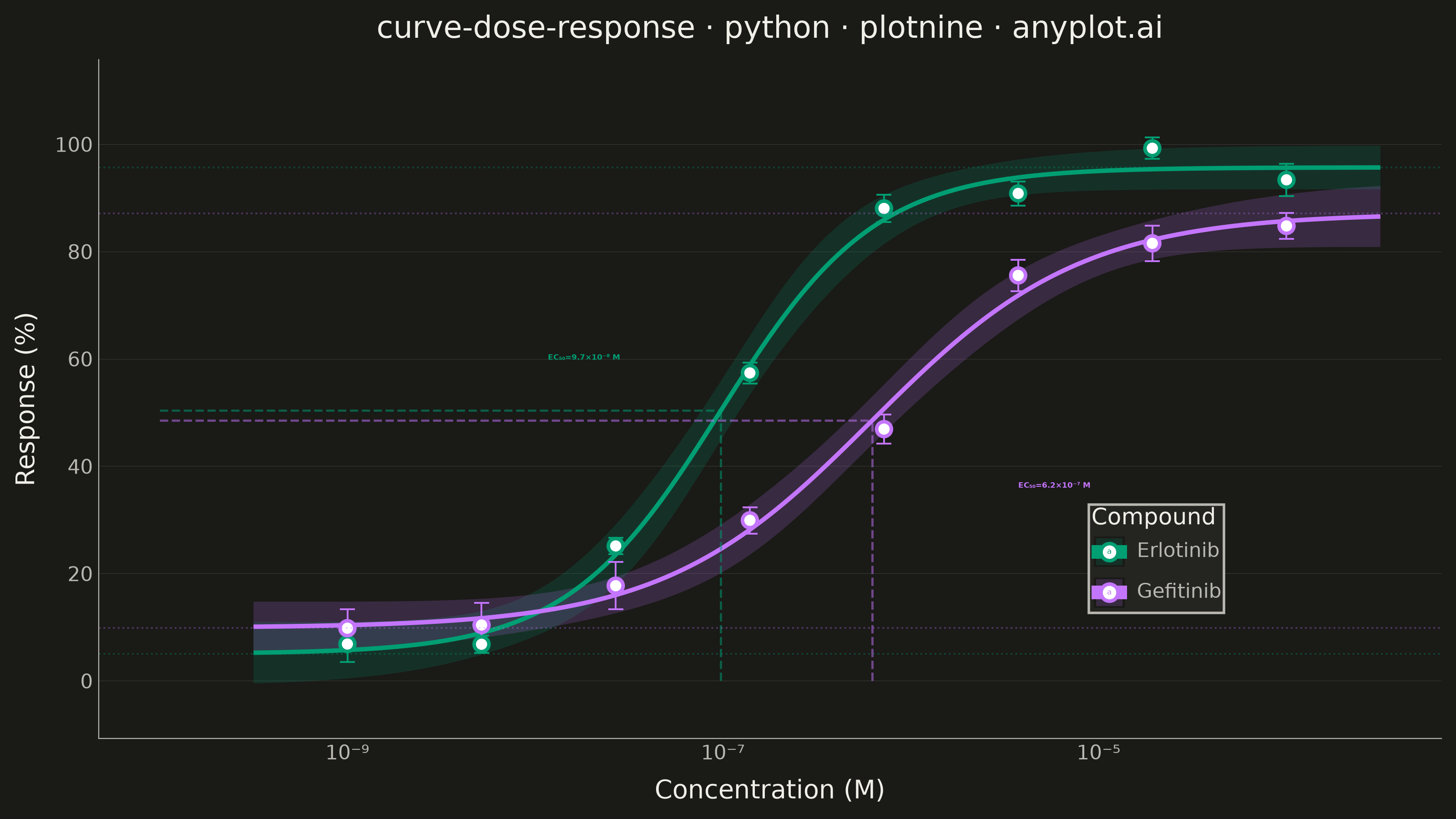
A sigmoidal dose-response curve that plots biological response against drug concentration on a logarithmic x-axis, fitted using a four-parameter logistic (4PL) model. This visualization is essential for determining drug potency metrics such as EC50 (half-maximal effective concentration) or IC50 (half-maximal inhibitory concentration), Hill slope steepness, and upper/lower response asymptotes. It enables rapid visual comparison of compound efficacy and is a standard tool in pharmacological analysis.
""" anyplot.ai
curve-dose-response: Pharmacological Dose-Response Curve
Library: plotnine 0.15.7 | Python 3.13.14
Quality: 91/100 | Updated: 2026-06-24
"""

import os

import numpy as np
import pandas as pd
from plotnine import (
    aes,
    element_blank,
    element_line,
    element_rect,
    element_text,
    geom_errorbar,
    geom_hline,
    geom_line,
    geom_point,
    geom_ribbon,
    geom_segment,
    geom_text,
    ggplot,
    guide_legend,
    guides,
    labs,
    scale_color_manual,
    scale_fill_manual,
    scale_x_log10,
    scale_y_continuous,
    theme,
    theme_minimal,
)
from scipy.optimize import curve_fit


# Theme tokens (Imprint palette — theme-adaptive chrome)
THEME = os.getenv("ANYPLOT_THEME", "light")
PAGE_BG = "#FAF8F1" if THEME == "light" else "#1A1A17"
ELEVATED_BG = "#FFFDF6" if THEME == "light" else "#242420"
INK = "#1A1A17" if THEME == "light" else "#F0EFE8"
INK_SOFT = "#4A4A44" if THEME == "light" else "#B8B7B0"

IMPRINT_PALETTE = ["#009E73", "#C475FD", "#4467A3", "#BD8233", "#AE3030", "#2ABCCD", "#954477", "#99B314"]

_SUP = str.maketrans("0123456789", "⁰¹²³⁴⁵⁶⁷⁸⁹")

# Data
np.random.seed(42)

concentrations = np.logspace(-9, -4, 8)
compounds = ["Erlotinib", "Gefitinib"]


def logistic_4pl(x, bottom, top, ec50, hill):
    return bottom + (top - bottom) / (1 + (ec50 / x) ** hill)


true_params = {
    "Erlotinib": {"bottom": 5, "top": 95, "ec50": 1e-7, "hill": 1.2},
    "Gefitinib": {"bottom": 10, "top": 85, "ec50": 5e-7, "hill": 0.9},
}

rows = []
for conc in concentrations:
    resp_a = logistic_4pl(conc, **true_params["Erlotinib"]) + np.random.normal(0, 3)
    resp_b = logistic_4pl(conc, **true_params["Gefitinib"]) + np.random.normal(0, 3.5)
    rows.append(
        {
            "concentration": conc,
            "response": resp_a,
            "response_sem": np.random.uniform(1.5, 4.0),
            "compound": "Erlotinib",
        }
    )
    rows.append(
        {
            "concentration": conc,
            "response": resp_b,
            "response_sem": np.random.uniform(2.0, 4.5),
            "compound": "Gefitinib",
        }
    )

df = pd.DataFrame(rows)

# Fit 4PL curves
fit_params = {}
for compound in compounds:
    subset = df[df["compound"] == compound]
    popt, pcov = curve_fit(
        logistic_4pl, subset["concentration"].values, subset["response"].values, p0=[5, 90, 1e-6, 1.0], maxfev=10000
    )
    fit_params[compound] = {"popt": popt, "pcov": pcov}

# Generate smooth fitted curves with 95% CI via delta method
conc_smooth = np.logspace(-9.5, -3.5, 200)
fit_rows = []
for compound, params in fit_params.items():
    popt = params["popt"]
    pcov = params["pcov"]
    fitted = logistic_4pl(conc_smooth, *popt)
    jacobian = np.zeros((len(conc_smooth), 4))
    eps = 1e-8
    for i in range(4):
        popt_up, popt_dn = popt.copy(), popt.copy()
        popt_up[i] += eps
        popt_dn[i] -= eps
        jacobian[:, i] = (logistic_4pl(conc_smooth, *popt_up) - logistic_4pl(conc_smooth, *popt_dn)) / (2 * eps)
    se = np.sqrt(np.maximum(np.sum(jacobian @ pcov * jacobian, axis=1), 0))
    for j, c in enumerate(conc_smooth):
        fit_rows.append(
            {
                "concentration": c,
                "fitted": fitted[j],
                "ci_lower": fitted[j] - 1.96 * se[j],
                "ci_upper": fitted[j] + 1.96 * se[j],
                "compound": compound,
            }
        )
df_fit = pd.DataFrame(fit_rows)

# EC50 reference data
colors = {"Erlotinib": IMPRINT_PALETTE[0], "Gefitinib": IMPRINT_PALETTE[1]}
ec50_rows = []
for compound, params in fit_params.items():
    bottom, top, ec50, hill = params["popt"]
    ec50_rows.append(
        {
            "compound": compound,
            "ec50": ec50,
            "half_response": bottom + (top - bottom) / 2,
            "bottom": bottom,
            "top": top,
            "x_start": 1e-10,
        }
    )
df_ec50 = pd.DataFrame(ec50_rows)

# EC50 annotation labels — staggered to prevent crowding
ec50_labels = []
for i, (_, row) in enumerate(df_ec50.iterrows()):
    ec50_val = row["ec50"]
    exp = int(np.floor(np.log10(ec50_val)))
    mantissa = ec50_val / 10**exp
    exp_str = str(abs(exp)).translate(_SUP)
    label = f"EC₅₀={mantissa:.1f}×10⁻{exp_str} M"
    # Erlotinib: left of EC50, above midpoint; Gefitinib: right of EC50, below midpoint
    x_pos = ec50_val * 0.12 if i == 0 else ec50_val * 6
    y_pos = row["half_response"] + 10 if i == 0 else row["half_response"] - 12
    ec50_labels.append({"concentration": x_pos, "response": y_pos, "label": label, "compound": row["compound"]})
df_ec50_labels = pd.DataFrame(ec50_labels)

# Plot
plot = (
    ggplot()
    + geom_ribbon(aes(x="concentration", ymin="ci_lower", ymax="ci_upper", fill="compound"), data=df_fit, alpha=0.18)
    + geom_line(aes(x="concentration", y="fitted", color="compound"), data=df_fit, size=1.0)
    + geom_errorbar(
        aes(x="concentration", ymin="response - response_sem", ymax="response + response_sem", color="compound"),
        data=df,
        width=0.08,
        size=0.4,
    )
    + geom_point(aes(x="concentration", y="response", color="compound"), data=df, size=2.5, fill="white", stroke=0.8)
)

# EC50 reference lines
for _, row in df_ec50.iterrows():
    col = colors[row["compound"]]
    rd = pd.DataFrame([row])
    plot = (
        plot
        + geom_segment(
            aes(x="ec50", xend="ec50", y=0, yend="half_response"),
            data=rd,
            linetype="dashed",
            color=col,
            size=0.5,
            alpha=0.5,
        )
        + geom_segment(
            aes(x="x_start", xend="ec50", y="half_response", yend="half_response"),
            data=rd,
            linetype="dashed",
            color=col,
            size=0.5,
            alpha=0.5,
        )
    )

# EC50 value annotations
plot = plot + geom_text(
    aes(x="concentration", y="response", label="label", color="compound"),
    data=df_ec50_labels,
    size=3.0,
    ha="left",
    fontweight="bold",
)

# Top/bottom asymptote reference lines
for _, row in df_ec50.iterrows():
    col = colors[row["compound"]]
    plot = (
        plot
        + geom_hline(yintercept=row["top"], linetype="dotted", color=col, size=0.4, alpha=0.3)
        + geom_hline(yintercept=row["bottom"], linetype="dotted", color=col, size=0.4, alpha=0.3)
    )

# Scales and style
plot = (
    plot
    + scale_x_log10(
        labels=lambda vals: [f"10⁻{str(abs(int(round(np.log10(v))))).translate(_SUP)}" if v > 0 else "" for v in vals]
    )
    + scale_y_continuous(breaks=range(0, 101, 20), limits=(-5, 110))
    + scale_color_manual(values=colors)
    + scale_fill_manual(values=colors)
    + labs(
        x="Concentration (M)",
        y="Response (%)",
        title="curve-dose-response · python · plotnine · anyplot.ai",
        color="Compound",
        fill="Compound",
    )
    + guides(color=guide_legend(override_aes={"size": 3}), fill=guide_legend(title="Compound"))
    + theme_minimal()
    + theme(
        figure_size=(8, 4.5),
        text=element_text(size=7, color=INK),
        axis_title=element_text(size=10, color=INK),
        axis_text=element_text(size=8, color=INK_SOFT),
        plot_title=element_text(size=12, color=INK),
        legend_title=element_text(size=9, color=INK),
        legend_text=element_text(size=8, color=INK_SOFT),
        legend_position=(0.82, 0.22),
        legend_background=element_rect(fill=ELEVATED_BG, color=INK_SOFT),
        legend_key_size=12,
        panel_grid_major_x=element_blank(),
        panel_grid_minor=element_blank(),
        panel_grid_major_y=element_line(color=INK, size=0.2, alpha=0.15),
        axis_line=element_line(color=INK_SOFT, size=0.4),
        plot_background=element_rect(fill=PAGE_BG, color=PAGE_BG),
        panel_background=element_rect(fill=PAGE_BG),
    )
)

# Save
plot.save(f"plot-{THEME}.png", dpi=400, width=8, height=4.5, units="in", verbose=False)
Runnable source as JSON, for any HTTP client: https://api.anyplot.ai/specs/curve-dose-response/plotnine/code. Any spec id and library id listed in llms-full.txt fit the same URL shape; every URL below is complete and callable.
{
  "spec_id": "curve-dose-response",
  "language": "python",
  "library": "plotnine",
  "page": "https://anyplot.ai/curve-dose-response/python/plotnine",
  "hub": "https://anyplot.ai/curve-dose-response",
  "code_json": "https://api.anyplot.ai/specs/curve-dose-response/plotnine/code",
  "spec_json": "https://api.anyplot.ai/specs/curve-dose-response",
  "render_light_png": "https://storage.googleapis.com/anyplot-images/plots/curve-dose-response/python/plotnine/plot-light.png",
  "render_dark_png": "https://storage.googleapis.com/anyplot-images/plots/curve-dose-response/python/plotnine/plot-dark.png",
  "quality_score": 91.0,
  "license": "MIT",
  "guide": "https://anyplot.ai/llms.txt"
}
Part of Pharmacological Dose-Response Curve on anyplot.ai.