Pharmacological Dose-Response Curve — D3.js

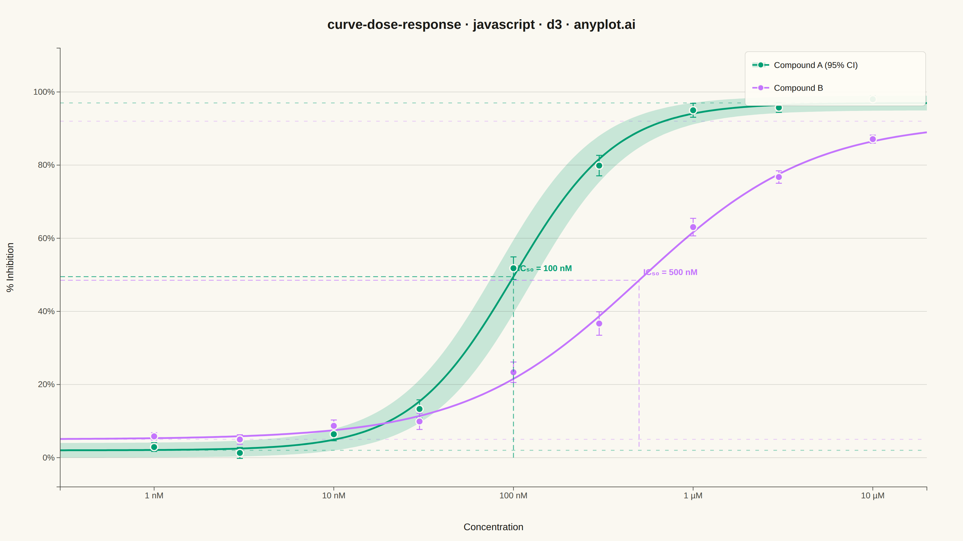
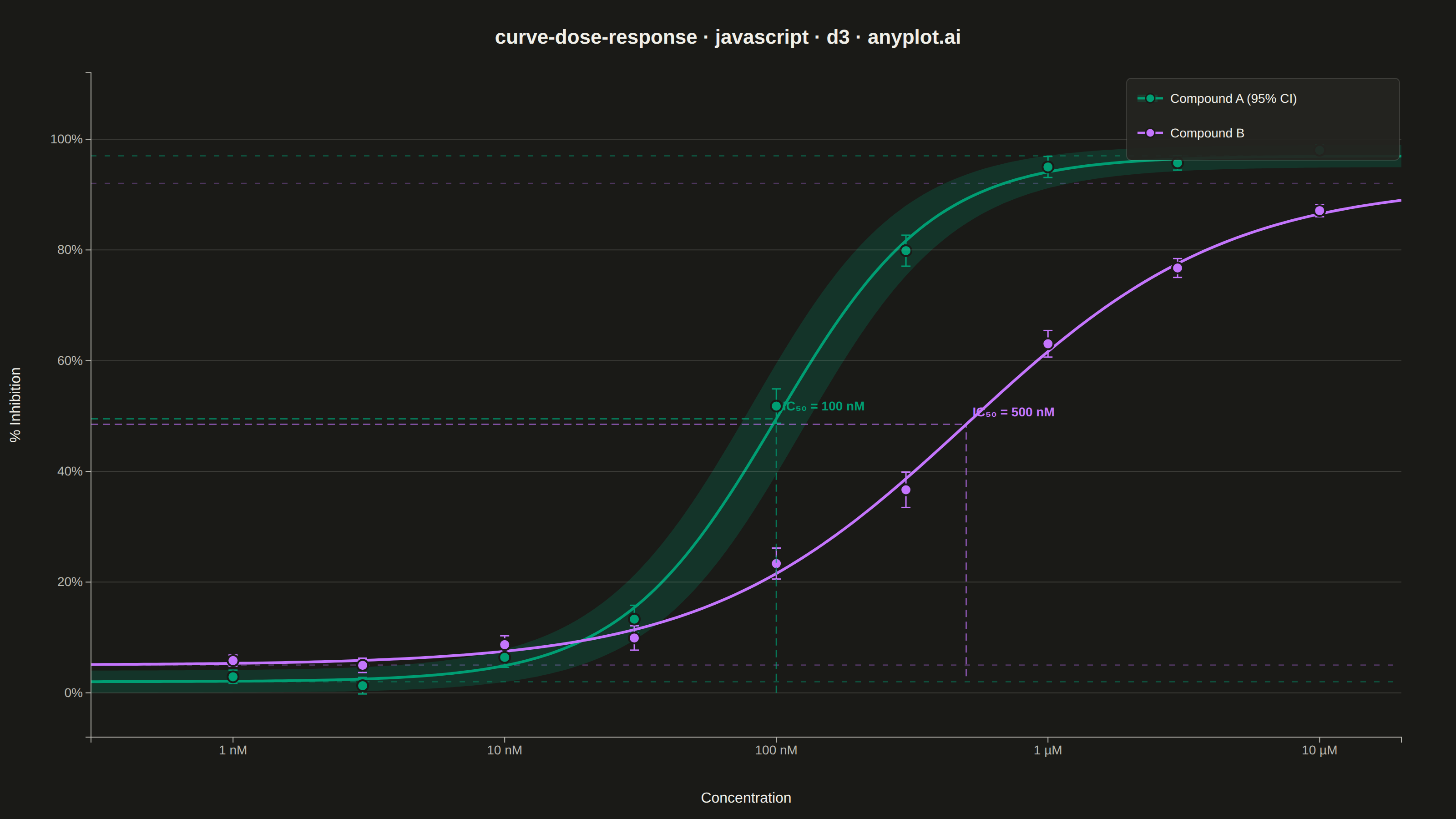
A sigmoidal dose-response curve that plots biological response against drug concentration on a logarithmic x-axis, fitted using a four-parameter logistic (4PL) model. This visualization is essential for determining drug potency metrics such as EC50 (half-maximal effective concentration) or IC50 (half-maximal inhibitory concentration), Hill slope steepness, and upper/lower response asymptotes. It enables rapid visual comparison of compound efficacy and is a standard tool in pharmacological analysis.

Renders

• Full-resolution render, light theme
• Full-resolution render, dark theme
• Interactive version, light theme
• Interactive version, dark theme

JavaScript source (D3.js)

// anyplot.ai
// curve-dose-response: Pharmacological Dose-Response Curve
// Library: d3 7.9.0 | JavaScript 22.22.3
// Quality: 89/100 | Created: 2026-06-24

const t = window.ANYPLOT_TOKENS;
const { width, height } = window.ANYPLOT_SIZE;

const margin = { top: 80, right: 60, bottom: 90, left: 100 };
const iw = width - margin.left - margin.right;
const ih = height - margin.top - margin.bottom;

// 4-parameter logistic model
function fourPL(conc, bottom, top, ec50, hill) {
  return bottom + (top - bottom) / (1 + Math.pow(ec50 / conc, hill));
}

// Compound parameters
const paramA = { name: "Compound A", bottom: 2, top: 97, ec50: 1e-7, hill: 1.5 };
const paramB = { name: "Compound B", bottom: 5, top: 92, ec50: 5e-7, hill: 0.9 };

// Hard-coded observed data points (deterministic)
const concPoints = [1e-9, 3e-9, 1e-8, 3e-8, 1e-7, 3e-7, 1e-6, 3e-6, 1e-5];
const noiseA   = [0.8, -1.2, 1.5, -2.1, 2.3, -1.8, 0.9, -0.7, 1.1];
const noiseB   = [0.5, -0.9, 1.2, -1.5, 1.8, -2.0, 1.4, -0.8, 0.6];
const semA     = [1.2,  1.5, 1.8,  2.5, 3.1,  2.8, 1.9,  1.3, 1.0];
const semB     = [1.0,  1.3, 1.6,  2.2, 2.8,  3.2, 2.4,  1.7, 1.1];

const dataA = concPoints.map((c, i) => ({
  conc: c,
  response: Math.min(100, Math.max(0,
    fourPL(c, paramA.bottom, paramA.top, paramA.ec50, paramA.hill) + noiseA[i])),
  sem: semA[i],
}));
const dataB = concPoints.map((c, i) => ({
  conc: c,
  response: Math.min(100, Math.max(0,
    fourPL(c, paramB.bottom, paramB.top, paramB.ec50, paramB.hill) + noiseB[i])),
  sem: semB[i],
}));

// Log-spaced smooth curve points
const nCurve = 200;
const logMin = Math.log10(3e-10);
const logMax = Math.log10(2e-5);
const curveConcList = d3.range(nCurve).map(i =>
  Math.pow(10, logMin + (logMax - logMin) * i / (nCurve - 1))
);

// CI half-width: bell-shaped, widest in the transition zone
function ciHalfWidth(response, bottom, top) {
  const p = (response - bottom) / (top - bottom);
  return 2.0 + 8.0 * 4 * p * (1 - p);
}

const curveA = curveConcList.map(c => {
  const resp = fourPL(c, paramA.bottom, paramA.top, paramA.ec50, paramA.hill);
  const w = ciHalfWidth(resp, paramA.bottom, paramA.top);
  return { conc: c, response: resp, lower: Math.max(-3, resp - w), upper: Math.min(103, resp + w) };
});
const curveB = curveConcList.map(c => ({
  conc: c,
  response: fourPL(c, paramB.bottom, paramB.top, paramB.ec50, paramB.hill),
}));

// Scales
const x = d3.scaleLog().domain([3e-10, 2e-5]).range([0, iw]);
const y = d3.scaleLinear().domain([-8, 112]).range([ih, 0]);

// SVG
const svg = d3.select("#container").append("svg").attr("width", width).attr("height", height);

svg.append("defs").append("clipPath").attr("id", "plot-clip")
  .append("rect").attr("width", iw).attr("height", ih);

const g = svg.append("g").attr("transform", `translate(${margin.left},${margin.top})`);
const clip = g.append("g").attr("clip-path", "url(#plot-clip)");

// Gridlines
[0, 20, 40, 60, 80, 100].forEach(yVal => {
  g.append("line")
    .attr("x1", 0).attr("x2", iw)
    .attr("y1", y(yVal)).attr("y2", y(yVal))
    .attr("stroke", t.grid).attr("stroke-width", 1);
});

// Asymptote dashed lines — Compound A
[paramA.top, paramA.bottom].forEach(aVal => {
  clip.append("line")
    .attr("x1", 0).attr("x2", iw)
    .attr("y1", y(aVal)).attr("y2", y(aVal))
    .attr("stroke", t.palette[0]).attr("stroke-dasharray", "6,9")
    .attr("stroke-width", 1.5).attr("opacity", 0.4);
});

// Asymptote dashed lines — Compound B
[paramB.top, paramB.bottom].forEach(aVal => {
  clip.append("line")
    .attr("x1", 0).attr("x2", iw)
    .attr("y1", y(aVal)).attr("y2", y(aVal))
    .attr("stroke", t.palette[1]).attr("stroke-dasharray", "6,9")
    .attr("stroke-width", 1.5).attr("opacity", 0.3);
});

// 95% CI band — Compound A
const areaGen = d3.area()
  .x(d => x(d.conc)).y0(d => y(d.lower)).y1(d => y(d.upper))
  .curve(d3.curveCatmullRom.alpha(0.5));

clip.append("path").datum(curveA)
  .attr("fill", t.palette[0]).attr("opacity", 0.20)
  .attr("d", areaGen);

// Fitted curves
const lineGen = d3.line().x(d => x(d.conc)).y(d => y(d.response))
  .curve(d3.curveCatmullRom.alpha(0.5));

clip.append("path").datum(curveA)
  .attr("fill", "none").attr("stroke", t.palette[0])
  .attr("stroke-width", 3).attr("d", lineGen);

clip.append("path").datum(curveB)
  .attr("fill", "none").attr("stroke", t.palette[1])
  .attr("stroke-width", 3).attr("d", lineGen);

// EC50 reference lines — Compound A
const ec50AResp = (paramA.bottom + paramA.top) / 2;
g.append("line")
  .attr("x1", x(paramA.ec50)).attr("x2", x(paramA.ec50))
  .attr("y1", y(paramA.bottom - 2)).attr("y2", y(ec50AResp))
  .attr("stroke", t.palette[0]).attr("stroke-dasharray", "8,5")
  .attr("stroke-width", 1.5).attr("opacity", 0.7);
g.append("line")
  .attr("x1", 0).attr("x2", x(paramA.ec50))
  .attr("y1", y(ec50AResp)).attr("y2", y(ec50AResp))
  .attr("stroke", t.palette[0]).attr("stroke-dasharray", "8,5")
  .attr("stroke-width", 1.5).attr("opacity", 0.7);

// EC50 reference lines — Compound B
const ec50BResp = (paramB.bottom + paramB.top) / 2;
g.append("line")
  .attr("x1", x(paramB.ec50)).attr("x2", x(paramB.ec50))
  .attr("y1", y(paramB.bottom - 2)).attr("y2", y(ec50BResp))
  .attr("stroke", t.palette[1]).attr("stroke-dasharray", "8,5")
  .attr("stroke-width", 1.5).attr("opacity", 0.6);
g.append("line")
  .attr("x1", 0).attr("x2", x(paramB.ec50))
  .attr("y1", y(ec50BResp)).attr("y2", y(ec50BResp))
  .attr("stroke", t.palette[1]).attr("stroke-dasharray", "8,5")
  .attr("stroke-width", 1.5).attr("opacity", 0.6);

// EC50 annotations
g.append("text")
  .attr("x", x(paramA.ec50) + 7).attr("y", y(ec50AResp) - 9)
  .attr("fill", t.palette[0]).style("font-size", "14px").style("font-weight", "600")
  .text("IC₅₀ = 100 nM");

g.append("text")
  .attr("x", x(paramB.ec50) + 7).attr("y", y(ec50BResp) - 9)
  .attr("fill", t.palette[1]).style("font-size", "14px").style("font-weight", "600")
  .text("IC₅₀ = 500 nM");

// Error bars — D3 data-join, inside clip group to respect plot boundary
const capW = 5;
[{ data: dataA, color: t.palette[0] }, { data: dataB, color: t.palette[1] }].forEach(({ data, color }) => {
  const ebG = clip.append("g");
  ebG.selectAll("line.stem").data(data).join("line")
    .attr("x1", d => x(d.conc)).attr("x2", d => x(d.conc))
    .attr("y1", d => y(d.response - d.sem)).attr("y2", d => y(d.response + d.sem))
    .attr("stroke", color).attr("stroke-width", 1.5);
  ebG.selectAll("line.cap-top").data(data).join("line")
    .attr("x1", d => x(d.conc) - capW).attr("x2", d => x(d.conc) + capW)
    .attr("y1", d => y(d.response + d.sem)).attr("y2", d => y(d.response + d.sem))
    .attr("stroke", color).attr("stroke-width", 1.5);
  ebG.selectAll("line.cap-bot").data(data).join("line")
    .attr("x1", d => x(d.conc) - capW).attr("x2", d => x(d.conc) + capW)
    .attr("y1", d => y(d.response - d.sem)).attr("y2", d => y(d.response - d.sem))
    .attr("stroke", color).attr("stroke-width", 1.5);
});

// Data points
clip.selectAll(".dot-a").data(dataA).join("circle")
  .attr("cx", d => x(d.conc)).attr("cy", d => y(d.response)).attr("r", 6)
  .attr("fill", t.palette[0]).attr("stroke", t.pageBg).attr("stroke-width", 2);

clip.selectAll(".dot-b").data(dataB).join("circle")
  .attr("cx", d => x(d.conc)).attr("cy", d => y(d.response)).attr("r", 6)
  .attr("fill", t.palette[1]).attr("stroke", t.pageBg).attr("stroke-width", 2);

// Axes
function xTickFormat(d) {
  const e = Math.round(Math.log10(d));
  const labels = { "-9": "1 nM", "-8": "10 nM", "-7": "100 nM", "-6": "1 µM", "-5": "10 µM" };
  return labels[String(e)] || "";
}

const xAxisG = g.append("g").attr("transform", `translate(0,${ih})`)
  .call(d3.axisBottom(x).tickValues([1e-9, 1e-8, 1e-7, 1e-6, 1e-5]).tickFormat(xTickFormat).tickSize(6));
xAxisG.selectAll("text").attr("fill", t.inkSoft).style("font-size", "14px");
xAxisG.selectAll("line").attr("stroke", t.inkSoft);
xAxisG.select(".domain").attr("stroke", t.inkSoft);

const yAxisG = g.append("g")
  .call(d3.axisLeft(y).tickValues([0, 20, 40, 60, 80, 100]).tickFormat(d => `${d}%`).tickSize(6));
yAxisG.selectAll("text").attr("fill", t.inkSoft).style("font-size", "14px");
yAxisG.selectAll("line").attr("stroke", t.inkSoft);
yAxisG.select(".domain").attr("stroke", t.inkSoft);

// Axis labels
svg.append("text")
  .attr("x", margin.left + iw / 2).attr("y", height - 18)
  .attr("text-anchor", "middle")
  .attr("fill", t.ink).style("font-size", "16px")
  .text("Concentration");

svg.append("text")
  .attr("transform", `translate(22,${margin.top + ih / 2}) rotate(-90)`)
  .attr("text-anchor", "middle")
  .attr("fill", t.ink).style("font-size", "16px")
  .text("% Inhibition");

// Legend — D3 data join
const legendEntries = [
  { name: "Compound A  (95% CI)", color: t.palette[0], hasCI: true },
  { name: "Compound B", color: t.palette[1], hasCI: false },
];

const lx = iw - 290;
const ly = 18;
const lPad = 12;
const lW = 300;
const lH = 90;
const rowH = 38;

g.append("rect")
  .attr("x", lx - lPad).attr("y", ly - lPad)
  .attr("width", lW).attr("height", lH)
  .attr("fill", t.elevatedBg).attr("rx", 5).attr("opacity", 0.92)
  .attr("stroke", t.grid).attr("stroke-width", 1);

const legendRows = g.selectAll(".legend-row").data(legendEntries).join("g")
  .attr("class", "legend-row")
  .attr("transform", (d, i) => `translate(${lx},${ly + i * rowH + 10})`);

legendRows.filter(d => d.hasCI).append("rect")
  .attr("x", 0).attr("y", -4).attr("width", 22).attr("height", 8)
  .attr("fill", d => d.color).attr("opacity", 0.20);

legendRows.append("line")
  .attr("x1", 0).attr("x2", 28)
  .attr("y1", 0).attr("y2", 0)
  .attr("stroke", d => d.color).attr("stroke-width", 2.5);

legendRows.append("circle")
  .attr("cx", 14).attr("cy", 0).attr("r", 5)
  .attr("fill", d => d.color).attr("stroke", t.pageBg).attr("stroke-width", 1.5);

legendRows.append("text")
  .attr("x", 36).attr("y", 5)
  .attr("fill", t.ink).style("font-size", "14px")
  .text(d => d.name);

// Title
svg.append("text")
  .attr("x", width / 2).attr("y", 48)
  .attr("text-anchor", "middle")
  .attr("fill", t.ink).style("font-size", "22px").style("font-weight", "600")
  .text("curve-dose-response · javascript · d3 · anyplot.ai");

Part of Pharmacological Dose-Response Curve on anyplot.ai.

Other implementations

• Pharmacological Dose-Response Curve in Chart.js (JavaScript)
• Pharmacological Dose-Response Curve in Apache ECharts (JavaScript)
• Pharmacological Dose-Response Curve in Highcharts (JavaScript)
• Pharmacological Dose-Response Curve in MUI X Charts (JavaScript)
• Pharmacological Dose-Response Curve in Makie.jl (Julia)
• Pharmacological Dose-Response Curve in Altair (Python)
• Pharmacological Dose-Response Curve in Bokeh (Python)
• Pharmacological Dose-Response Curve in lets-plot (Python)
• Pharmacological Dose-Response Curve in Matplotlib (Python)
• Pharmacological Dose-Response Curve in Plotly (Python)
• Pharmacological Dose-Response Curve in plotnine (Python)
• Pharmacological Dose-Response Curve in Pygal (Python)
• Pharmacological Dose-Response Curve in Seaborn (Python)
• Pharmacological Dose-Response Curve in ggplot2 (R)