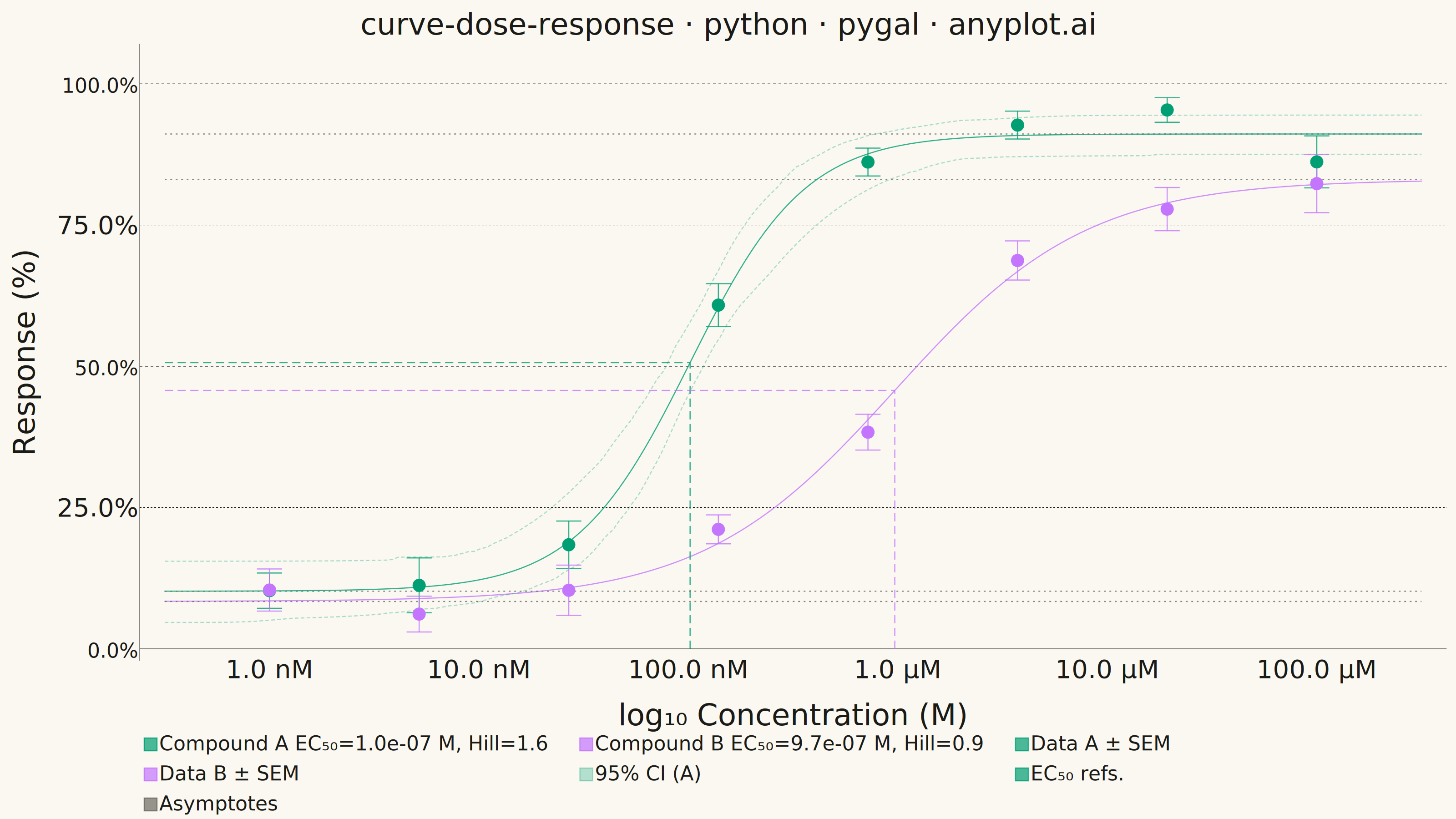
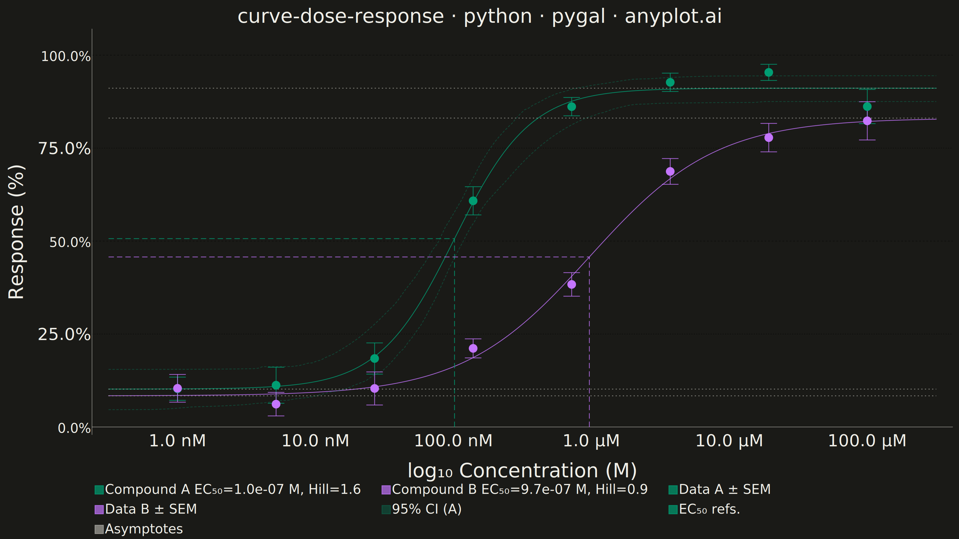
A sigmoidal dose-response curve that plots biological response against drug concentration on a logarithmic x-axis, fitted using a four-parameter logistic (4PL) model. This visualization is essential for determining drug potency metrics such as EC50 (half-maximal effective concentration) or IC50 (half-maximal inhibitory concentration), Hill slope steepness, and upper/lower response asymptotes. It enables rapid visual comparison of compound efficacy and is a standard tool in pharmacological analysis.
""" anyplot.ai
curve-dose-response: Pharmacological Dose-Response Curve
Library: pygal 3.1.3 | Python 3.13.15
Quality: 94/100 | Updated: 2026-08-17
"""

import os

import cairosvg
import numpy as np
import pygal
from pygal.style import Style
from scipy.optimize import curve_fit


# Theme tokens
THEME = os.getenv("ANYPLOT_THEME", "light")
PAGE_BG = "#FAF8F1" if THEME == "light" else "#1A1A17"
INK = "#1A1A17" if THEME == "light" else "#F0EFE8"
INK_MUTED = "#6B6A63" if THEME == "light" else "#A8A79F"

# Imprint palette — first two categorical positions
C_A = "#009E73"  # Compound A — Imprint brand green
C_B = "#C475FD"  # Compound B — Imprint lavender
# 95% CI band color-coded to Compound A using RGBA CSS color (pygal SVG feature)
CI_A = "rgba(0, 158, 115, 0.40)"

# Palette tuple matches series add order (11 series total)
CHART_COLORS = (
    C_A,  # 1: Compound A fitted curve
    C_B,  # 2: Compound B fitted curve
    C_A,  # 3: Data points A
    C_B,  # 4: Data points B
    CI_A,  # 5: 95% CI upper (color-coded to Compound A, semi-transparent)
    CI_A,  # 6: 95% CI lower (None label)
    C_A,  # 7: EC50 reference A
    C_B,  # 8: EC50 reference B (None label)
    INK_MUTED,  # 9: Asymptotes (structural, very subtle)
    C_A,  # 10: Error bars A (None label)
    C_B,  # 11: Error bars B (None label)
)


def four_pl(x, bottom, top, ec50, hill):
    return bottom + (top - bottom) / (1 + (ec50 / x) ** hill)


def fmt_concentration(log_val):
    """Format log10 concentration to human-readable units for interactive tooltips."""
    val = 10 ** float(log_val)
    if val >= 1e-6:
        return f"{val * 1e6:.1f} µM"
    if val >= 1e-9:
        return f"{val * 1e9:.1f} nM"
    return f"{val * 1e12:.1f} pM"


# Data
np.random.seed(42)
concentrations = np.logspace(-9, -4, 8)
log_conc = np.log10(concentrations)

# Compound A — potent agonist (EC50 ~100 nM)
response_a_true = four_pl(concentrations, 5, 95, 1e-7, 1.2)
response_a_sem = np.random.uniform(2, 5, len(concentrations))
response_a = response_a_true + np.random.normal(0, response_a_sem)

# Compound B — moderate agonist (EC50 ~1 µM)
response_b_true = four_pl(concentrations, 10, 85, 1e-6, 0.9)
response_b_sem = np.random.uniform(2, 6, len(concentrations))
response_b = response_b_true + np.random.normal(0, response_b_sem)

# Fit 4PL curves
popt_a, pcov_a = curve_fit(four_pl, concentrations, response_a, p0=[0, 100, 1e-7, 1], maxfev=10000)
popt_b, pcov_b = curve_fit(four_pl, concentrations, response_b, p0=[0, 100, 1e-6, 1], maxfev=10000)

# Smooth curves for plotting
conc_smooth = np.logspace(-9.5, -3.5, 200)
log_smooth = np.log10(conc_smooth)
fit_a = four_pl(conc_smooth, *popt_a)
fit_b = four_pl(conc_smooth, *popt_b)

# Extract parameters
bottom_a, top_a, ec50_a, hill_a = popt_a
bottom_b, top_b, ec50_b, hill_b = popt_b
half_a = bottom_a + (top_a - bottom_a) / 2
half_b = bottom_b + (top_b - bottom_b) / 2
log_ec50_a = np.log10(ec50_a)
log_ec50_b = np.log10(ec50_b)

# 95% CI for Compound A via covariance sampling
np.random.seed(99)
param_samples = np.random.multivariate_normal(popt_a, pcov_a, size=200)
fit_ensemble = np.array([four_pl(conc_smooth, *p) for p in param_samples])
ci_lower = np.percentile(fit_ensemble, 2.5, axis=0)
ci_upper = np.percentile(fit_ensemble, 97.5, axis=0)

# Title (49 chars < 67 baseline → keep full title_font_size=66)
title = "curve-dose-response · python · pygal · anyplot.ai"

# Style — canonical pygal sizing for 3200×1800 canvas
custom_style = Style(
    background=PAGE_BG,
    plot_background=PAGE_BG,
    foreground=INK,
    foreground_strong=INK,
    foreground_subtle=INK_MUTED,
    colors=CHART_COLORS,
    title_font_size=66,
    label_font_size=56,
    major_label_font_size=44,
    legend_font_size=44,
    value_font_size=36,
    stroke_width=2.5,
    font_family="sans-serif",
)

# Chart
chart = pygal.XY(
    width=3200,
    height=1800,
    style=custom_style,
    title=title,
    x_title="log₁₀ Concentration (M)",
    y_title="Response (%)",
    show_dots=False,
    stroke=True,
    show_x_guides=False,
    show_y_guides=True,
    legend_at_bottom=True,
    legend_at_bottom_columns=3,
    legend_box_size=28,
    x_label_rotation=0,
    truncate_legend=-1,
    range=(0, 105),
    allow_interruptions=True,
    js=[],
    print_values=False,
    value_formatter=lambda y: f"{y:.1f}%",
    x_value_formatter=fmt_concentration,
)

# Restrict y-axis ticks to 5 clean quartile levels — reduces grid clutter
chart.y_labels = [0, 25, 50, 75, 100]

# Fitted curves (solid, prominent — primary data layer)
chart.add(
    f"Compound A  EC₅₀={ec50_a:.1e} M, Hill={hill_a:.1f}",
    list(zip(log_smooth.tolist(), fit_a.tolist(), strict=True)),
    show_dots=False,
    stroke_style={"width": 8, "linecap": "round", "linejoin": "round"},
)
chart.add(
    f"Compound B  EC₅₀={ec50_b:.1e} M, Hill={hill_b:.1f}",
    list(zip(log_smooth.tolist(), fit_b.tolist(), strict=True)),
    show_dots=False,
    stroke_style={"width": 8, "linecap": "round", "linejoin": "round"},
)

# Data points (scatter, no connecting line)
chart.add(
    "Data A ± SEM",
    list(zip(log_conc.tolist(), response_a.tolist(), strict=True)),
    stroke=False,
    show_dots=True,
    dots_size=14,
)
chart.add(
    "Data B ± SEM",
    list(zip(log_conc.tolist(), response_b.tolist(), strict=True)),
    stroke=False,
    show_dots=True,
    dots_size=14,
)

# 95% CI bounds for Compound A — color-coded to Compound A via RGBA semi-transparent stroke
chart.add(
    "95% CI (A)",
    list(zip(log_smooth.tolist(), ci_upper.tolist(), strict=True)),
    show_dots=False,
    stroke_style={"width": 3, "dasharray": "8, 5"},
)
chart.add(
    None,
    list(zip(log_smooth.tolist(), ci_lower.tolist(), strict=True)),
    show_dots=False,
    stroke_style={"width": 3, "dasharray": "8, 5"},
)

# EC50 reference lines — vertical + horizontal crosshair per compound
chart.add(
    "EC₅₀ refs.",
    [(log_ec50_a, 0), (log_ec50_a, half_a), None, (log_smooth[0], half_a), (log_ec50_a, half_a)],
    show_dots=False,
    dots_size=0,
    stroke_style={"width": 3, "dasharray": "18, 10"},
)
chart.add(
    None,
    [(log_ec50_b, 0), (log_ec50_b, half_b), None, (log_smooth[0], half_b), (log_ec50_b, half_b)],
    show_dots=False,
    dots_size=0,
    stroke_style={"width": 3, "dasharray": "18, 10"},
)

# Asymptote lines (very fine dash — background reference only)
x_lo, x_hi = log_smooth[0], log_smooth[-1]
chart.add(
    "Asymptotes",
    [
        (x_lo, top_a),
        (x_hi, top_a),
        None,
        (x_lo, bottom_a),
        (x_hi, bottom_a),
        None,
        (x_lo, top_b),
        (x_hi, top_b),
        None,
        (x_lo, bottom_b),
        (x_hi, bottom_b),
    ],
    show_dots=False,
    dots_size=0,
    stroke_style={"width": 1.5, "dasharray": "4, 8"},
)

# Error bars — stems and caps
cap = 0.06
for resp, sem in [(response_a, response_a_sem), (response_b, response_b_sem)]:
    pts = []
    for i in range(len(log_conc)):
        x = log_conc[i]
        lo = resp[i] - sem[i]
        hi = resp[i] + sem[i]
        pts.extend([(x, lo), (x, hi), None, (x - cap, lo), (x + cap, lo), None, (x - cap, hi), (x + cap, hi), None])
    chart.add(None, pts, stroke=True, show_dots=False, dots_size=0, stroke_style={"width": 2})

# Save
svg = chart.render(is_unicode=True)
with open(f"plot-{THEME}.html", "w", encoding="utf-8") as f:
    f.write(svg)
cairosvg.svg2png(bytestring=svg.encode("utf-8"), write_to=f"plot-{THEME}.png", dpi=96)
Runnable source as JSON, for any HTTP client: https://api.anyplot.ai/specs/curve-dose-response/pygal/code. Any spec id and library id listed in llms-full.txt fit the same URL shape; every URL below is complete and callable.
{
  "spec_id": "curve-dose-response",
  "language": "python",
  "library": "pygal",
  "page": "https://anyplot.ai/curve-dose-response/python/pygal",
  "hub": "https://anyplot.ai/curve-dose-response",
  "code_json": "https://api.anyplot.ai/specs/curve-dose-response/pygal/code",
  "spec_json": "https://api.anyplot.ai/specs/curve-dose-response",
  "render_light_png": "https://storage.googleapis.com/anyplot-images/plots/curve-dose-response/python/pygal/plot-light.png",
  "render_dark_png": "https://storage.googleapis.com/anyplot-images/plots/curve-dose-response/python/pygal/plot-dark.png",
  "interactive_light_html": "https://storage.googleapis.com/anyplot-images/plots/curve-dose-response/python/pygal/plot-light.html",
  "interactive_dark_html": "https://storage.googleapis.com/anyplot-images/plots/curve-dose-response/python/pygal/plot-dark.html",
  "quality_score": 94.0,
  "license": "MIT",
  "guide": "https://anyplot.ai/llms.txt"
}
Part of Pharmacological Dose-Response Curve on anyplot.ai.