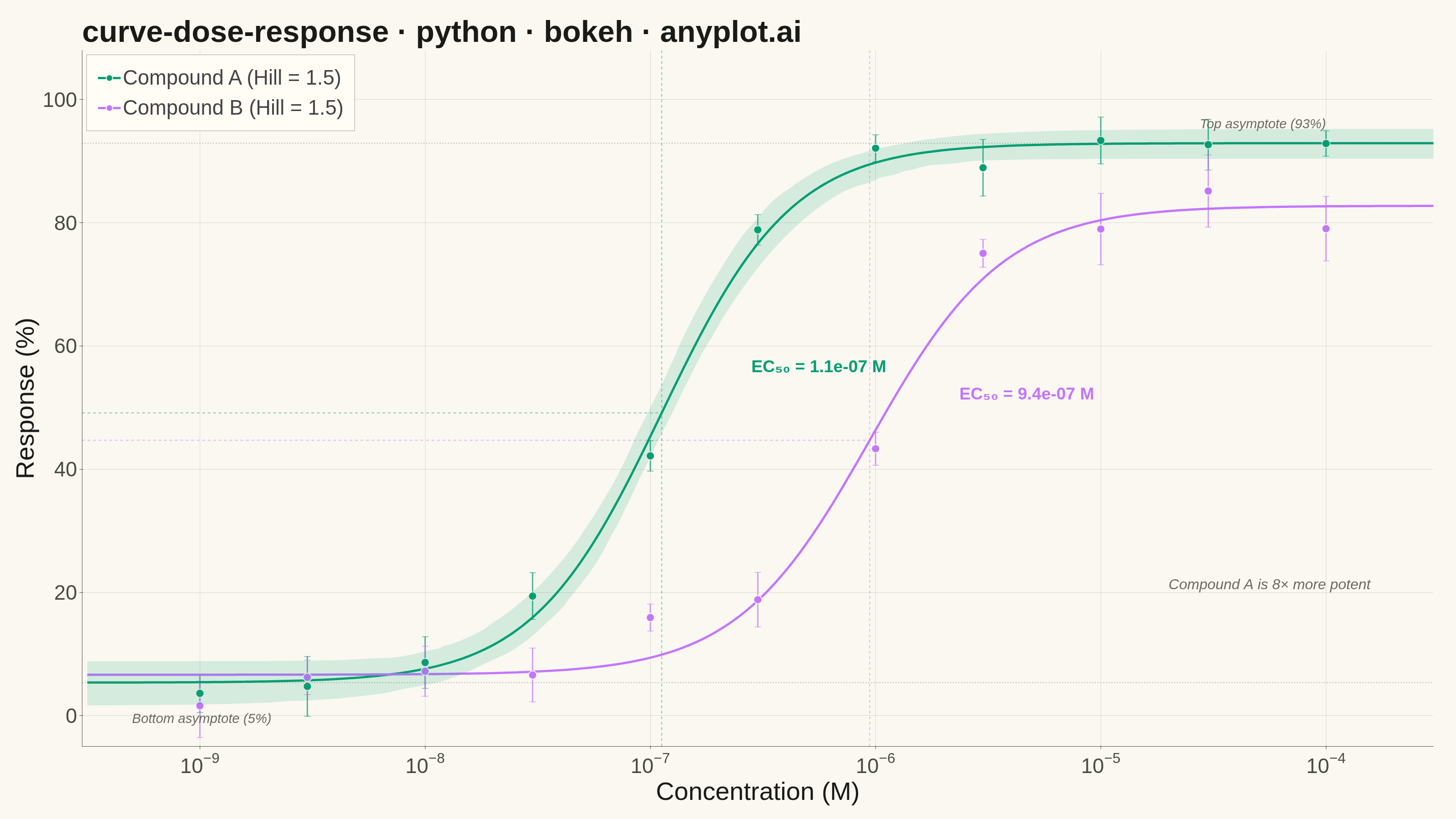
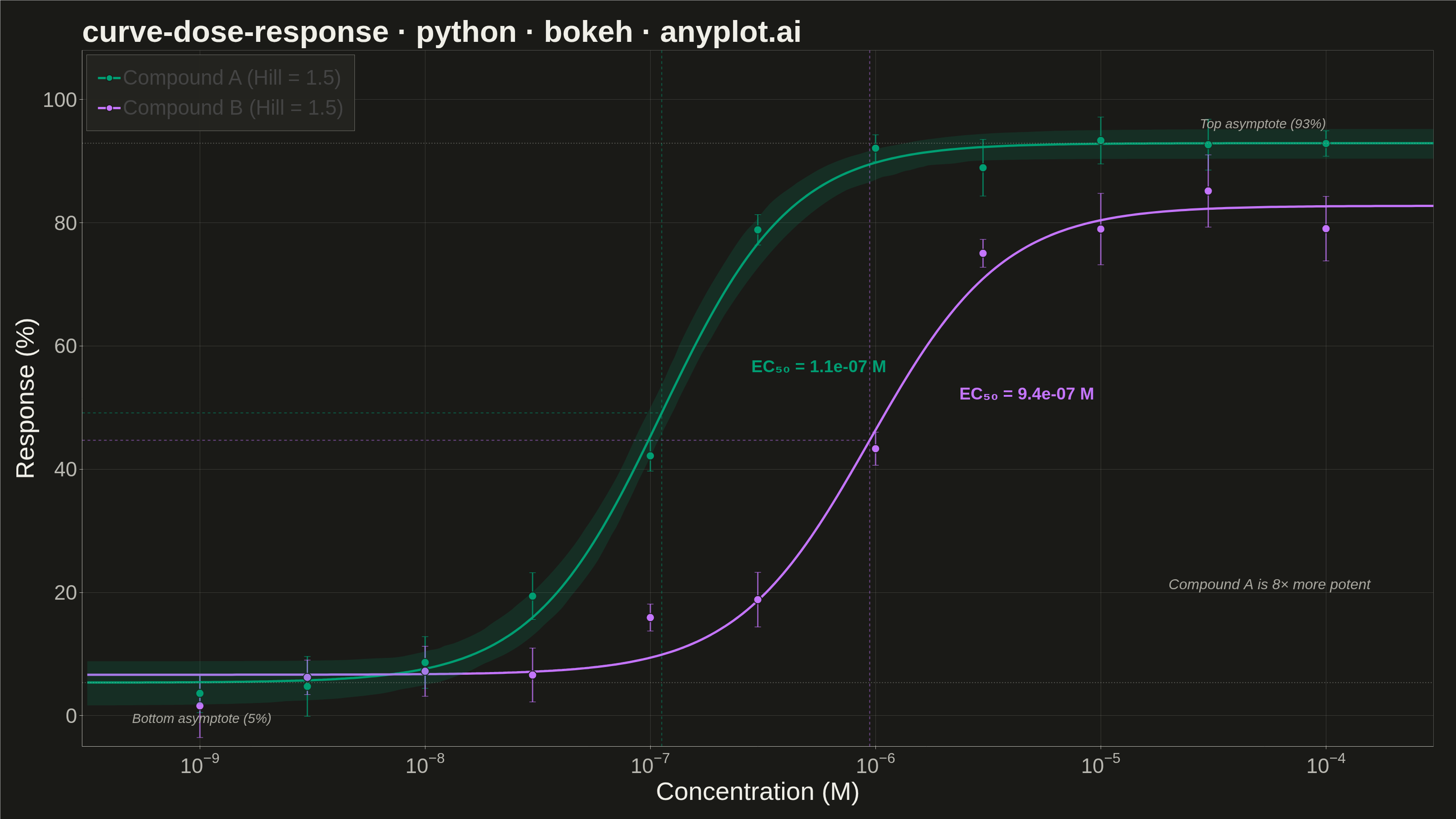
A sigmoidal dose-response curve that plots biological response against drug concentration on a logarithmic x-axis, fitted using a four-parameter logistic (4PL) model. This visualization is essential for determining drug potency metrics such as EC50 (half-maximal effective concentration) or IC50 (half-maximal inhibitory concentration), Hill slope steepness, and upper/lower response asymptotes. It enables rapid visual comparison of compound efficacy and is a standard tool in pharmacological analysis.
""" anyplot.ai
curve-dose-response: Pharmacological Dose-Response Curve
Library: bokeh 3.9.1 | Python 3.13.14
Quality: 88/100 | Updated: 2026-06-24
"""

import os
import time
from pathlib import Path

import numpy as np
from bokeh.io import output_file, save
from bokeh.models import Band, ColumnDataSource, Label, Legend, LegendItem, Span, Whisker
from bokeh.plotting import figure
from scipy.optimize import curve_fit
from selenium import webdriver
from selenium.webdriver.chrome.options import Options


# Theme tokens (Imprint palette — see default-style-guide.md)
THEME = os.getenv("ANYPLOT_THEME", "light")
PAGE_BG = "#FAF8F1" if THEME == "light" else "#1A1A17"
ELEVATED_BG = "#FFFDF6" if THEME == "light" else "#242420"
INK = "#1A1A17" if THEME == "light" else "#F0EFE8"
INK_SOFT = "#4A4A44" if THEME == "light" else "#B8B7B0"
INK_MUTED = "#6B6A63" if THEME == "light" else "#A8A79F"

# Imprint categorical palette — first series always #009E73
COLOR_A = "#009E73"  # brand green — Compound A
COLOR_B = "#C475FD"  # lavender — Compound B

# Data
np.random.seed(42)

concentrations = np.array([1e-9, 3e-9, 1e-8, 3e-8, 1e-7, 3e-7, 1e-6, 3e-6, 1e-5, 3e-5, 1e-4])


def logistic_4pl(x, bottom, top, ec50, hill):
    return bottom + (top - bottom) / (1 + (ec50 / x) ** hill)


# Compound A — potent agonist with EC50 ~100 nM
true_params_a = [5, 95, 1e-7, 1.2]
response_a_mean = logistic_4pl(concentrations, *true_params_a)
response_a_sem = np.random.uniform(2, 5, len(concentrations))
response_a_raw = response_a_mean + np.random.normal(0, 3, len(concentrations))

# Compound B — less potent agonist with EC50 ~1 µM
true_params_b = [8, 85, 1e-6, 1.5]
response_b_mean = logistic_4pl(concentrations, *true_params_b)
response_b_sem = np.random.uniform(2, 6, len(concentrations))
response_b_raw = response_b_mean + np.random.normal(0, 3, len(concentrations))

# Fit 4PL to noisy data
popt_a, pcov_a = curve_fit(logistic_4pl, concentrations, response_a_raw, p0=[0, 100, 1e-7, 1], maxfev=10000)
popt_b, pcov_b = curve_fit(logistic_4pl, concentrations, response_b_raw, p0=[0, 100, 1e-6, 1], maxfev=10000)

# Smooth fitted curves
conc_smooth = np.logspace(-9.5, -3.5, 300)
fit_a = logistic_4pl(conc_smooth, *popt_a)
fit_b = logistic_4pl(conc_smooth, *popt_b)

# 95% CI for Compound A via parameter covariance sampling
n_samples = 200
ci_samples = np.zeros((n_samples, len(conc_smooth)))
for i in range(n_samples):
    sampled_params = np.random.multivariate_normal(popt_a, pcov_a)
    ci_samples[i] = logistic_4pl(conc_smooth, *sampled_params)
ci_lower_a = np.percentile(ci_samples, 2.5, axis=0)
ci_upper_a = np.percentile(ci_samples, 97.5, axis=0)

# EC50 and half-response values from fitted parameters
ec50_a = popt_a[2]
ec50_b = popt_b[2]
half_response_a = popt_a[0] + (popt_a[1] - popt_a[0]) / 2
half_response_b = popt_b[0] + (popt_b[1] - popt_b[0]) / 2
fold_diff = ec50_b / ec50_a

# Plot — 3200×1800 canonical landscape canvas
title = "curve-dose-response · python · bokeh · anyplot.ai"

p = figure(
    width=3200,
    height=1800,
    title=title,
    x_axis_label="Concentration (M)",
    y_axis_label="Response (%)",
    x_axis_type="log",
    x_range=(3e-10, 3e-4),
    y_range=(-5, 108),
    toolbar_location=None,
    min_border_bottom=160,
    min_border_left=180,
    min_border_top=110,
    min_border_right=50,
)

# Confidence band — Compound A 95% CI
band_source = ColumnDataSource(data={"conc": conc_smooth, "lower": ci_lower_a, "upper": ci_upper_a})
band = Band(
    base="conc",
    lower="lower",
    upper="upper",
    source=band_source,
    fill_alpha=0.15,
    fill_color=COLOR_A,
    line_color=COLOR_A,
    line_alpha=0.0,
)
p.add_layout(band)

# Fitted curves
source_a = ColumnDataSource(data={"conc": conc_smooth, "response": fit_a})
source_b = ColumnDataSource(data={"conc": conc_smooth, "response": fit_b})
line_a = p.line("conc", "response", source=source_a, line_width=5, line_color=COLOR_A)
line_b = p.line("conc", "response", source=source_b, line_width=5, line_color=COLOR_B)

# Data points with SEM error bars
pts_source_a = ColumnDataSource(
    data={
        "conc": concentrations,
        "response": response_a_raw,
        "upper": response_a_raw + response_a_sem,
        "lower": response_a_raw - response_a_sem,
    }
)
pts_source_b = ColumnDataSource(
    data={
        "conc": concentrations,
        "response": response_b_raw,
        "upper": response_b_raw + response_b_sem,
        "lower": response_b_raw - response_b_sem,
    }
)

whisker_a = Whisker(
    base="conc", upper="upper", lower="lower", source=pts_source_a, line_color=COLOR_A, line_width=3, line_alpha=0.7
)
whisker_a.upper_head.line_color = COLOR_A
whisker_a.upper_head.size = 14
whisker_a.lower_head.line_color = COLOR_A
whisker_a.lower_head.size = 14
p.add_layout(whisker_a)

whisker_b = Whisker(
    base="conc", upper="upper", lower="lower", source=pts_source_b, line_color=COLOR_B, line_width=3, line_alpha=0.7
)
whisker_b.upper_head.line_color = COLOR_B
whisker_b.upper_head.size = 14
whisker_b.lower_head.line_color = COLOR_B
whisker_b.lower_head.size = 14
p.add_layout(whisker_b)

scatter_a = p.scatter("conc", "response", source=pts_source_a, size=18, color=COLOR_A, line_color=PAGE_BG, line_width=2)
scatter_b = p.scatter("conc", "response", source=pts_source_b, size=18, color=COLOR_B, line_color=PAGE_BG, line_width=2)

# EC50 reference lines — Compound A
ec50_vline_a = Span(
    location=ec50_a, dimension="height", line_color=COLOR_A, line_width=2, line_dash="dashed", line_alpha=0.5
)
p.add_layout(ec50_vline_a)
ec50_hline_src_a = ColumnDataSource(data={"x": [3e-10, ec50_a], "y": [half_response_a, half_response_a]})
p.line("x", "y", source=ec50_hline_src_a, line_color=COLOR_A, line_width=2, line_dash="dashed", line_alpha=0.5)

# EC50 reference lines — Compound B
ec50_vline_b = Span(
    location=ec50_b, dimension="height", line_color=COLOR_B, line_width=2, line_dash="dashed", line_alpha=0.5
)
p.add_layout(ec50_vline_b)
ec50_hline_src_b = ColumnDataSource(data={"x": [3e-10, ec50_b], "y": [half_response_b, half_response_b]})
p.line("x", "y", source=ec50_hline_src_b, line_color=COLOR_B, line_width=2, line_dash="dashed", line_alpha=0.5)

# Asymptote reference lines (Compound A)
top_asymptote = Span(
    location=popt_a[1], dimension="width", line_color=INK_MUTED, line_width=2, line_dash="dotted", line_alpha=0.5
)
bottom_asymptote = Span(
    location=popt_a[0], dimension="width", line_color=INK_MUTED, line_width=2, line_dash="dotted", line_alpha=0.5
)
p.add_layout(top_asymptote)
p.add_layout(bottom_asymptote)

# Asymptote labels
top_asym_label = Label(
    x=1e-4,
    y=popt_a[1] + 2,
    text=f"Top asymptote ({popt_a[1]:.0f}%)",
    text_font_size="22pt",
    text_color=INK_MUTED,
    text_font_style="italic",
    text_align="right",
)
bottom_asym_label = Label(
    x=5e-10,
    y=popt_a[0] - 7,
    text=f"Bottom asymptote ({popt_a[0]:.0f}%)",
    text_font_size="22pt",
    text_color=INK_MUTED,
    text_font_style="italic",
)
p.add_layout(top_asym_label)
p.add_layout(bottom_asym_label)

# EC50 annotations
ec50_a_label = Label(
    x=ec50_a * 2.5,
    y=half_response_a + 6,
    text=f"EC₅₀ = {ec50_a:.1e} M",
    text_font_size="28pt",
    text_color=COLOR_A,
    text_font_style="bold",
)
ec50_b_label = Label(
    x=ec50_b * 2.5,
    y=half_response_b + 6,
    text=f"EC₅₀ = {ec50_b:.1e} M",
    text_font_size="28pt",
    text_color=COLOR_B,
    text_font_style="bold",
)
p.add_layout(ec50_a_label)
p.add_layout(ec50_b_label)

# Potency comparison annotation
potency_label = Label(
    x=2e-5,
    y=20,
    text=f"Compound A is {fold_diff:.0f}× more potent",
    text_font_size="24pt",
    text_color=INK_MUTED,
    text_font_style="italic",
)
p.add_layout(potency_label)

# Legend — top-left avoids crowding near the plateau (top-right)
legend = Legend(
    items=[
        LegendItem(label="Compound A (Hill = {:.1f})".format(popt_a[3]), renderers=[line_a, scatter_a]),
        LegendItem(label="Compound B (Hill = {:.1f})".format(popt_b[3]), renderers=[line_b, scatter_b]),
    ],
    location="top_left",
)
legend.label_text_font_size = "34pt"
legend.background_fill_color = ELEVATED_BG
legend.background_fill_alpha = 0.95
legend.border_line_color = INK_SOFT
legend.border_line_width = 1
legend.spacing = 14
legend.padding = 24
legend.glyph_width = 50
legend.glyph_height = 36
p.add_layout(legend)

# Style — theme-adaptive chrome (canonical bokeh sizing: 50pt / 42pt / 34pt)
p.title.text_font_size = "50pt"
p.title.text_font_style = "bold"
p.title.text_color = INK

p.xaxis.axis_label_text_font_size = "42pt"
p.yaxis.axis_label_text_font_size = "42pt"
p.xaxis.axis_label_text_color = INK
p.yaxis.axis_label_text_color = INK
p.xaxis.axis_label_text_font_style = "normal"
p.yaxis.axis_label_text_font_style = "normal"

p.xaxis.major_label_text_font_size = "34pt"
p.yaxis.major_label_text_font_size = "34pt"
p.xaxis.major_label_text_color = INK_SOFT
p.yaxis.major_label_text_color = INK_SOFT

p.background_fill_color = PAGE_BG
p.border_fill_color = PAGE_BG
p.outline_line_color = None

p.xaxis.axis_line_color = INK_SOFT
p.yaxis.axis_line_color = INK_SOFT
p.xaxis.major_tick_line_color = INK_SOFT
p.yaxis.major_tick_line_color = INK_SOFT
p.xaxis.minor_tick_line_color = None
p.yaxis.minor_tick_line_color = None

p.xgrid.grid_line_alpha = 0.15
p.ygrid.grid_line_alpha = 0.15
p.xgrid.grid_line_color = INK
p.ygrid.grid_line_color = INK

# Save — HTML interactive artifact + Selenium PNG screenshot
output_file(f"plot-{THEME}.html")
save(p)

W, H = 3200, 1800
opts = Options()
for arg in (
    "--headless=new",
    "--no-sandbox",
    "--disable-dev-shm-usage",
    "--disable-gpu",
    f"--window-size={W},{H}",
    "--hide-scrollbars",
):
    opts.add_argument(arg)
driver = webdriver.Chrome(options=opts)
# Override viewport to exact canvas dimensions (window size includes browser chrome)
driver.execute_cdp_cmd(
    "Emulation.setDeviceMetricsOverride", {"mobile": False, "width": W, "height": H, "deviceScaleFactor": 1}
)
driver.get(f"file://{Path(f'plot-{THEME}.html').resolve()}")
time.sleep(3)
driver.save_screenshot(f"plot-{THEME}.png")
driver.quit()
Runnable source as JSON, for any HTTP client: https://api.anyplot.ai/specs/curve-dose-response/bokeh/code. Any spec id and library id listed in llms-full.txt fit the same URL shape; every URL below is complete and callable.
{
  "spec_id": "curve-dose-response",
  "language": "python",
  "library": "bokeh",
  "page": "https://anyplot.ai/curve-dose-response/python/bokeh",
  "hub": "https://anyplot.ai/curve-dose-response",
  "code_json": "https://api.anyplot.ai/specs/curve-dose-response/bokeh/code",
  "spec_json": "https://api.anyplot.ai/specs/curve-dose-response",
  "render_light_png": "https://storage.googleapis.com/anyplot-images/plots/curve-dose-response/python/bokeh/plot-light.png",
  "render_dark_png": "https://storage.googleapis.com/anyplot-images/plots/curve-dose-response/python/bokeh/plot-dark.png",
  "interactive_light_html": "https://storage.googleapis.com/anyplot-images/plots/curve-dose-response/python/bokeh/plot-light.html",
  "interactive_dark_html": "https://storage.googleapis.com/anyplot-images/plots/curve-dose-response/python/bokeh/plot-dark.html",
  "quality_score": 88.0,
  "license": "MIT",
  "guide": "https://anyplot.ai/llms.txt"
}
Part of Pharmacological Dose-Response Curve on anyplot.ai.