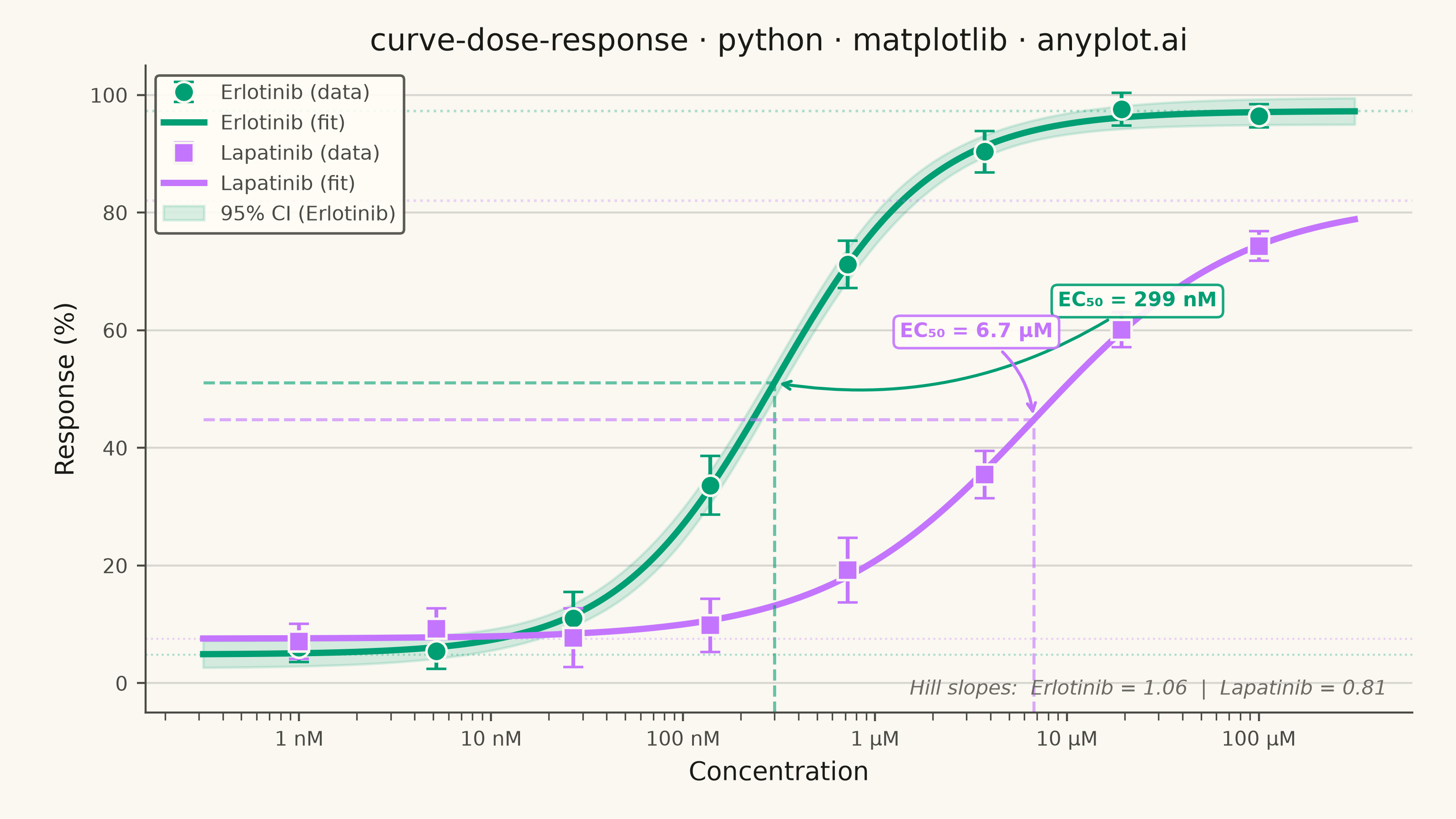
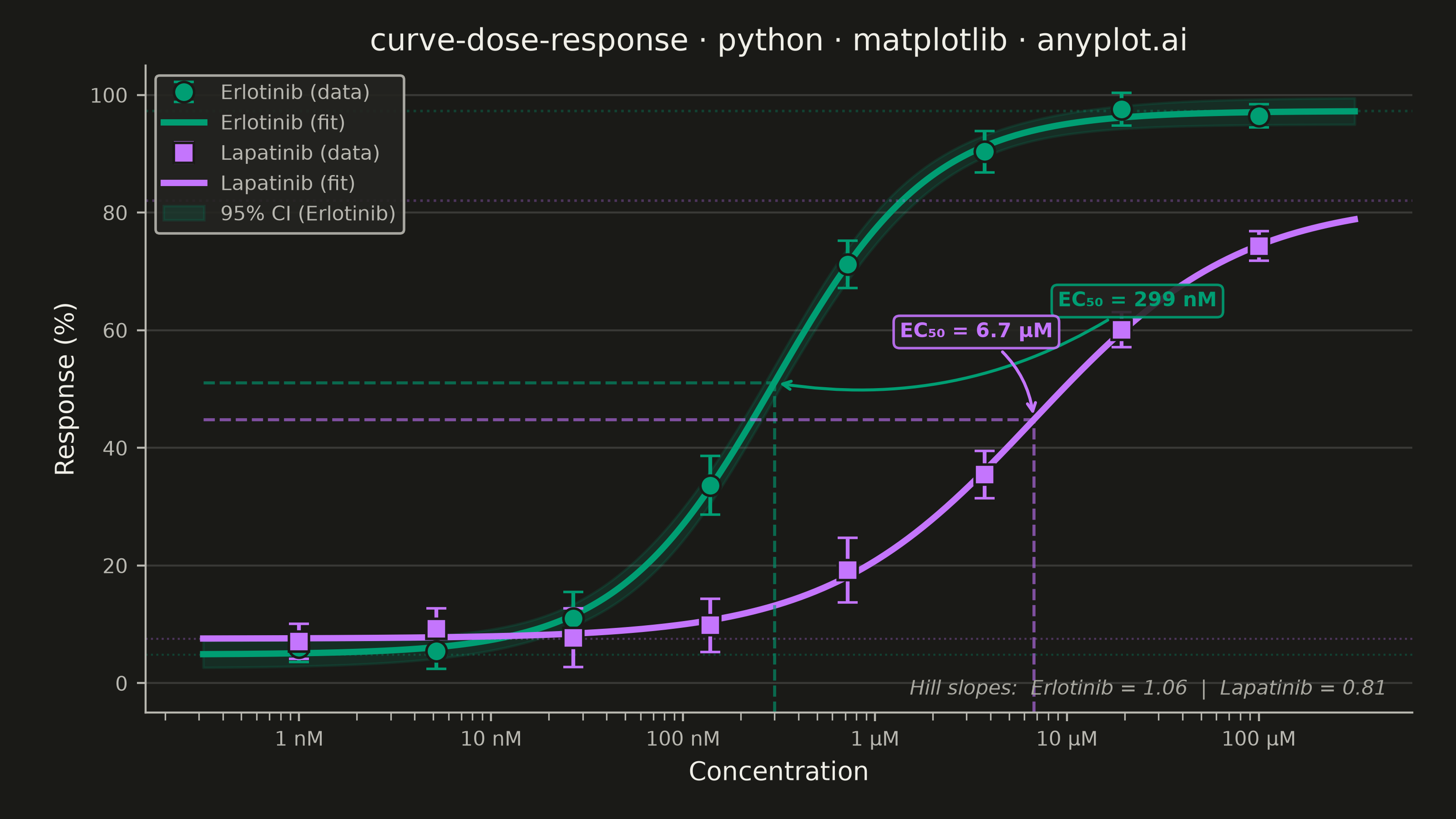
A sigmoidal dose-response curve that plots biological response against drug concentration on a logarithmic x-axis, fitted using a four-parameter logistic (4PL) model. This visualization is essential for determining drug potency metrics such as EC50 (half-maximal effective concentration) or IC50 (half-maximal inhibitory concentration), Hill slope steepness, and upper/lower response asymptotes. It enables rapid visual comparison of compound efficacy and is a standard tool in pharmacological analysis.
""" anyplot.ai
curve-dose-response: Pharmacological Dose-Response Curve
Library: matplotlib 3.11.0 | Python 3.13.14
Quality: 90/100 | Updated: 2026-06-24
"""

import os

import matplotlib.pyplot as plt
import matplotlib.ticker as ticker
import numpy as np
from scipy.optimize import curve_fit
from scipy.stats import t as t_dist


# Theme tokens — Imprint palette chrome
THEME = os.getenv("ANYPLOT_THEME", "light")
PAGE_BG = "#FAF8F1" if THEME == "light" else "#1A1A17"
ELEVATED_BG = "#FFFDF6" if THEME == "light" else "#242420"
INK = "#1A1A17" if THEME == "light" else "#F0EFE8"
INK_SOFT = "#4A4A44" if THEME == "light" else "#B8B7B0"
INK_MUTED = "#6B6A63" if THEME == "light" else "#A8A79F"

# Imprint palette — positions 1 and 2
COLORS = ["#009E73", "#C475FD"]

# Data
np.random.seed(42)
concentrations = np.logspace(-9, -4, 8)

drug_names = ["Erlotinib", "Lapatinib"]
bottom_a, top_a, ec50_a, hill_a = 5.0, 95.0, 3e-7, 1.2
bottom_b, top_b, ec50_b, hill_b = 8.0, 80.0, 5e-6, 0.9


def logistic4pl(conc, bottom, top, ec50, hill):
    return bottom + (top - bottom) / (1 + (ec50 / conc) ** hill)


response_a_true = logistic4pl(concentrations, bottom_a, top_a, ec50_a, hill_a)
response_b_true = logistic4pl(concentrations, bottom_b, top_b, ec50_b, hill_b)

sem_a = np.array([2.5, 3.0, 4.5, 5.0, 4.0, 3.5, 2.8, 2.0])
sem_b = np.array([3.0, 3.5, 5.0, 4.5, 5.5, 4.0, 3.0, 2.5])

response_a = response_a_true + np.random.normal(0, 2, len(concentrations))
response_b = response_b_true + np.random.normal(0, 2, len(concentrations))

# Fit 4PL curves
popt_a, pcov_a = curve_fit(logistic4pl, concentrations, response_a, p0=[5, 95, 1e-7, 1.0], maxfev=10000)
popt_b, pcov_b = curve_fit(logistic4pl, concentrations, response_b, p0=[8, 80, 1e-6, 1.0], maxfev=10000)

conc_smooth = np.logspace(-9.5, -3.5, 300)
fit_a = logistic4pl(conc_smooth, *popt_a)
fit_b = logistic4pl(conc_smooth, *popt_b)

# 95% CI for Erlotinib via delta method with covariance propagation
n_params = len(popt_a)
n_data = len(concentrations)
dof = max(n_data - n_params, 1)
t_val = t_dist.ppf(0.975, dof)

delta = 1e-8 * np.abs(popt_a) + 1e-15
jacobian_a = np.zeros((len(conc_smooth), n_params))
for i in range(n_params):
    params_up = popt_a.copy()
    params_up[i] += delta[i]
    params_dn = popt_a.copy()
    params_dn[i] -= delta[i]
    jacobian_a[:, i] = (logistic4pl(conc_smooth, *params_up) - logistic4pl(conc_smooth, *params_dn)) / (2 * delta[i])

pred_var_a = np.sum(jacobian_a @ pcov_a * jacobian_a, axis=1)
pred_se_a = np.sqrt(np.maximum(pred_var_a, 0))
ci_lower_a = fit_a - t_val * pred_se_a
ci_upper_a = fit_a + t_val * pred_se_a

# Fitted EC50 and half-maximal response values
ec50_fit_a = popt_a[2]
ec50_fit_b = popt_b[2]
half_response_a = popt_a[0] + (popt_a[1] - popt_a[0]) / 2
half_response_b = popt_b[0] + (popt_b[1] - popt_b[0]) / 2

# EC50 label strings (inlined — no separate function)
ec50_label_a = f"EC₅₀ = {ec50_fit_a * 1e9:.0f} nM" if ec50_fit_a < 1e-6 else f"EC₅₀ = {ec50_fit_a * 1e6:.1f} µM"
ec50_label_b = f"EC₅₀ = {ec50_fit_b * 1e9:.0f} nM" if ec50_fit_b < 1e-6 else f"EC₅₀ = {ec50_fit_b * 1e6:.1f} µM"

# Plot
title = "curve-dose-response · python · matplotlib · anyplot.ai"
title_fontsize = max(8, round(12 * 67 / len(title))) if len(title) > 67 else 12

fig, ax = plt.subplots(figsize=(8, 4.5), dpi=400, facecolor=PAGE_BG)
ax.set_facecolor(PAGE_BG)
ax.set_ylim(-5, 105)

ax.fill_between(conc_smooth, ci_lower_a, ci_upper_a, alpha=0.15, color=COLORS[0], label=f"95% CI ({drug_names[0]})")
ax.plot(conc_smooth, fit_a, linewidth=2.5, color=COLORS[0], label=f"{drug_names[0]} (fit)")
ax.plot(conc_smooth, fit_b, linewidth=2.5, color=COLORS[1], label=f"{drug_names[1]} (fit)")

ax.errorbar(
    concentrations,
    response_a,
    yerr=sem_a,
    fmt="o",
    markersize=8,
    color=COLORS[0],
    markeredgecolor=PAGE_BG,
    markeredgewidth=1.0,
    elinewidth=1.5,
    capsize=4,
    capthick=1.5,
    zorder=5,
    label=f"{drug_names[0]} (data)",
)
ax.errorbar(
    concentrations,
    response_b,
    yerr=sem_b,
    fmt="s",
    markersize=8,
    color=COLORS[1],
    markeredgecolor=PAGE_BG,
    markeredgewidth=1.0,
    elinewidth=1.5,
    capsize=4,
    capthick=1.5,
    zorder=5,
    label=f"{drug_names[1]} (data)",
)

# EC50 reference lines
ax.hlines(half_response_a, conc_smooth[0], ec50_fit_a, linestyles="dashed", colors=COLORS[0], linewidth=1.2, alpha=0.6)
ax.vlines(ec50_fit_a, -5, half_response_a, linestyles="dashed", colors=COLORS[0], linewidth=1.2, alpha=0.6)
ax.hlines(half_response_b, conc_smooth[0], ec50_fit_b, linestyles="dashed", colors=COLORS[1], linewidth=1.2, alpha=0.6)
ax.vlines(ec50_fit_b, -5, half_response_b, linestyles="dashed", colors=COLORS[1], linewidth=1.2, alpha=0.6)

# Top and bottom asymptote markers
ax.axhline(y=popt_a[1], linestyle=":", color=COLORS[0], alpha=0.3, linewidth=1.0)
ax.axhline(y=popt_b[1], linestyle=":", color=COLORS[1], alpha=0.3, linewidth=1.0)
ax.axhline(y=popt_a[0], linestyle=":", color=COLORS[0], alpha=0.3, linewidth=0.8)
ax.axhline(y=popt_b[0], linestyle=":", color=COLORS[1], alpha=0.3, linewidth=0.8)

# EC50 callout annotations with theme-adaptive boxes
ax.annotate(
    ec50_label_a,
    xy=(ec50_fit_a, half_response_a),
    xytext=(ec50_fit_a * 30, half_response_a + 13),
    fontsize=8,
    fontweight="bold",
    color=COLORS[0],
    arrowprops={"arrowstyle": "->", "color": COLORS[0], "lw": 1.2, "connectionstyle": "arc3,rad=-0.2"},
    bbox={"boxstyle": "round,pad=0.3", "facecolor": ELEVATED_BG, "edgecolor": COLORS[0], "alpha": 0.9},
    zorder=10,
)
ax.annotate(
    ec50_label_b,
    xy=(ec50_fit_b, half_response_b),
    xytext=(ec50_fit_b / 5, half_response_b + 14),
    fontsize=8,
    fontweight="bold",
    color=COLORS[1],
    arrowprops={"arrowstyle": "->", "color": COLORS[1], "lw": 1.2, "connectionstyle": "arc3,rad=-0.25"},
    bbox={"boxstyle": "round,pad=0.3", "facecolor": ELEVATED_BG, "edgecolor": COLORS[1], "alpha": 0.9},
    zorder=10,
)

# Hill slope footer
ax.text(
    0.98,
    0.02,
    f"Hill slopes:  {drug_names[0]} = {popt_a[3]:.2f}  |  {drug_names[1]} = {popt_b[3]:.2f}",
    transform=ax.transAxes,
    fontsize=8,
    color=INK_MUTED,
    ha="right",
    va="bottom",
    style="italic",
)

# Style
ax.set_xscale("log")
ax.set_xlabel("Concentration", fontsize=10, color=INK)
ax.set_ylabel("Response (%)", fontsize=10, color=INK)
ax.set_title(title, fontsize=title_fontsize, fontweight="medium", color=INK)
ax.tick_params(axis="both", labelsize=8, colors=INK_SOFT, labelcolor=INK_SOFT)
ax.spines["top"].set_visible(False)
ax.spines["right"].set_visible(False)
for s in ("left", "bottom"):
    ax.spines[s].set_color(INK_SOFT)
ax.yaxis.grid(True, alpha=0.15, linewidth=0.8, color=INK)

# Custom concentration formatter — shows nM below 1 µM, µM above
ax.xaxis.set_major_formatter(
    ticker.FuncFormatter(lambda x, _: f"{x * 1e9:.0f} nM" if x < 1e-6 else f"{x * 1e6:.0f} µM")
)
ax.xaxis.set_minor_locator(ticker.LogLocator(base=10.0, subs=np.arange(2, 10) * 0.1, numticks=50))
ax.xaxis.set_minor_formatter(ticker.NullFormatter())
ax.tick_params(axis="x", which="minor", length=3, width=0.6, colors=INK_SOFT)

# Legend — reordered: A data, A fit, B data, B fit, CI band
handles, labels_list = ax.get_legend_handles_labels()
order = [3, 1, 4, 2, 0]
leg = ax.legend(
    [handles[i] for i in order], [labels_list[i] for i in order], fontsize=8, loc="upper left", framealpha=0.9
)
leg.get_frame().set_facecolor(ELEVATED_BG)
leg.get_frame().set_edgecolor(INK_SOFT)
plt.setp(leg.get_texts(), color=INK_SOFT)

fig.subplots_adjust(left=0.10, right=0.97, top=0.92, bottom=0.13)

# Save
plt.savefig(f"plot-{THEME}.png", dpi=400, facecolor=PAGE_BG)
Runnable source as JSON, for any HTTP client: https://api.anyplot.ai/specs/curve-dose-response/matplotlib/code. Any spec id and library id listed in llms-full.txt fit the same URL shape; every URL below is complete and callable.
{
  "spec_id": "curve-dose-response",
  "language": "python",
  "library": "matplotlib",
  "page": "https://anyplot.ai/curve-dose-response/python/matplotlib",
  "hub": "https://anyplot.ai/curve-dose-response",
  "code_json": "https://api.anyplot.ai/specs/curve-dose-response/matplotlib/code",
  "spec_json": "https://api.anyplot.ai/specs/curve-dose-response",
  "render_light_png": "https://storage.googleapis.com/anyplot-images/plots/curve-dose-response/python/matplotlib/plot-light.png",
  "render_dark_png": "https://storage.googleapis.com/anyplot-images/plots/curve-dose-response/python/matplotlib/plot-dark.png",
  "quality_score": 90.0,
  "license": "MIT",
  "guide": "https://anyplot.ai/llms.txt"
}
Part of Pharmacological Dose-Response Curve on anyplot.ai.