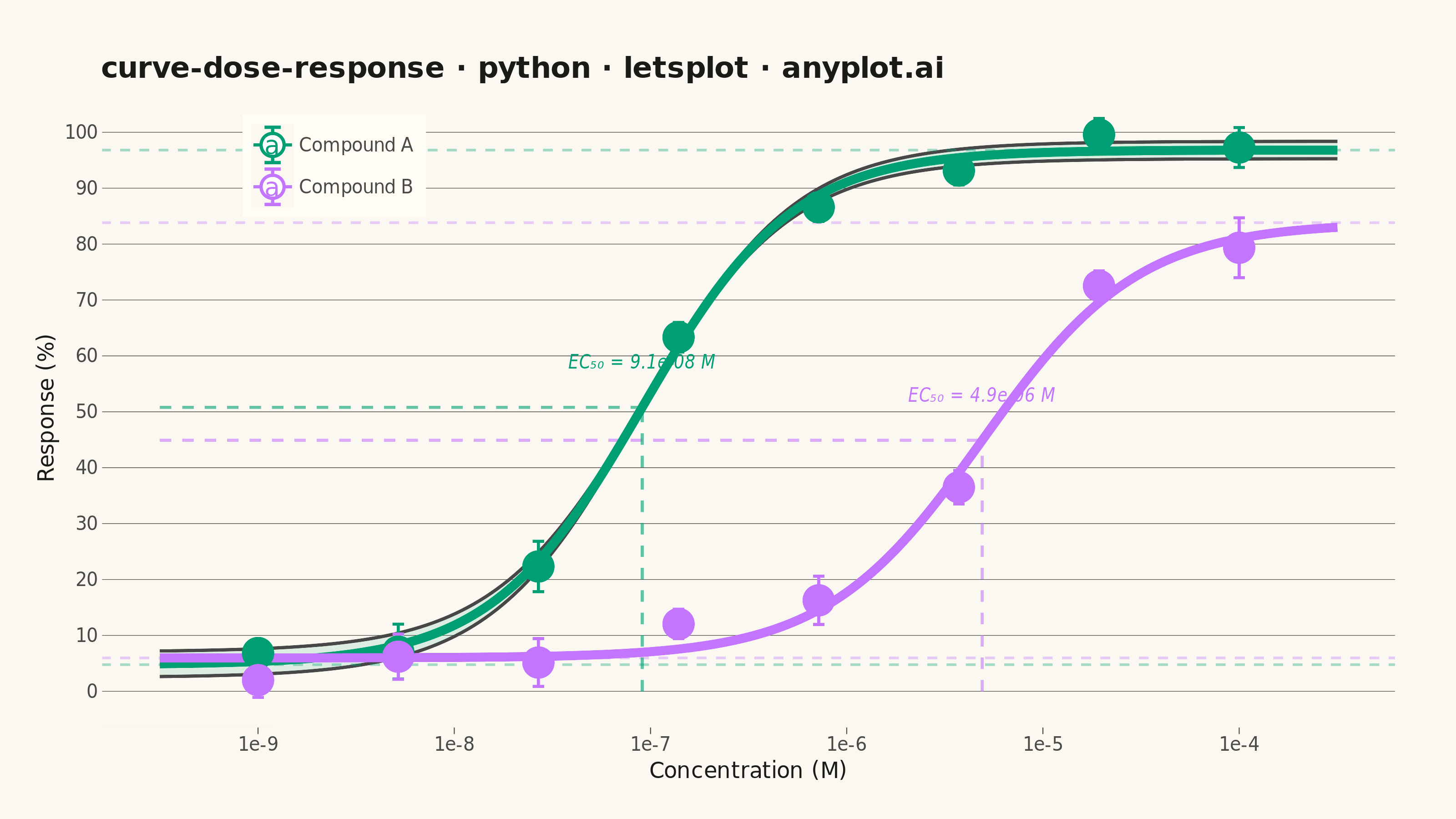
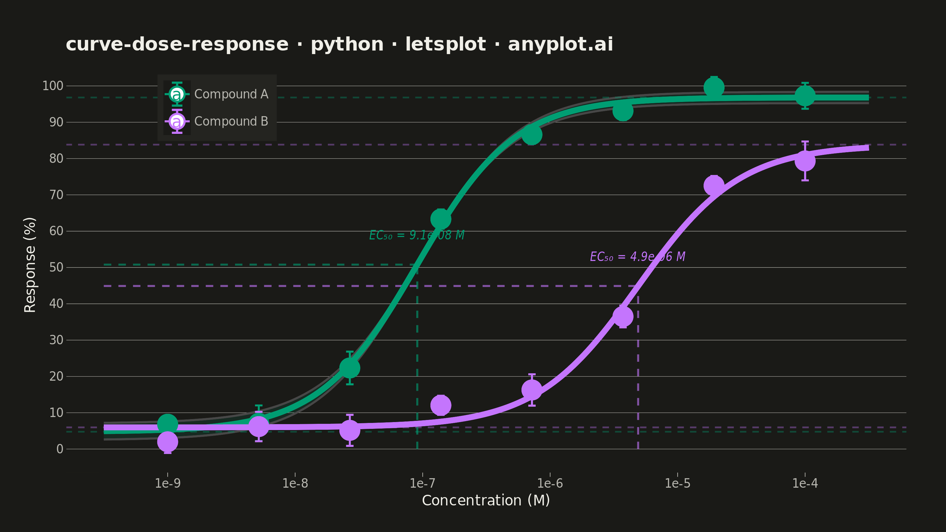
A sigmoidal dose-response curve that plots biological response against drug concentration on a logarithmic x-axis, fitted using a four-parameter logistic (4PL) model. This visualization is essential for determining drug potency metrics such as EC50 (half-maximal effective concentration) or IC50 (half-maximal inhibitory concentration), Hill slope steepness, and upper/lower response asymptotes. It enables rapid visual comparison of compound efficacy and is a standard tool in pharmacological analysis.
""" anyplot.ai
curve-dose-response: Pharmacological Dose-Response Curve
Library: letsplot 4.10.1 | Python 3.13.14
Quality: 90/100 | Updated: 2026-06-24
"""

import os

import numpy as np
import pandas as pd
from lets_plot import *
from scipy.optimize import curve_fit


LetsPlot.setup_html()

# Theme tokens (see prompts/default-style-guide.md "Theme-adaptive Chrome")
THEME = os.getenv("ANYPLOT_THEME", "light")
PAGE_BG = "#FAF8F1" if THEME == "light" else "#1A1A17"
ELEVATED_BG = "#FFFDF6" if THEME == "light" else "#242420"
INK = "#1A1A17" if THEME == "light" else "#F0EFE8"
INK_SOFT = "#4A4A44" if THEME == "light" else "#B8B7B0"

# Imprint palette — first series always #009E73
IMPRINT_PALETTE = ["#009E73", "#C475FD", "#4467A3", "#BD8233", "#AE3030", "#2ABCCD", "#954477", "#99B314"]
COLOR_A = IMPRINT_PALETTE[0]  # brand green — Compound A
COLOR_B = IMPRINT_PALETTE[1]  # lavender — Compound B

# Data — synthetic dose-response for two pharmacological compounds
np.random.seed(42)
concentrations = np.logspace(-9, -4, 8)

# 4PL model: response = Bottom + (Top - Bottom) / (1 + (EC50/conc)^Hill)
four_pl = lambda conc, bottom, top, ec50, hill: bottom + (top - bottom) / (1 + (ec50 / conc) ** hill)

# Compound A — high potency, steep Hill slope
bottom_a, top_a, ec50_a, hill_a = 5.0, 95.0, 1e-7, 1.2
response_a = four_pl(concentrations, bottom_a, top_a, ec50_a, hill_a)
response_a_noisy = response_a + np.random.normal(0, 3, len(concentrations))
sem_a = np.random.uniform(2, 5, len(concentrations))

# Compound B — lower potency, shallower Hill slope
bottom_b, top_b, ec50_b, hill_b = 8.0, 85.0, 5e-6, 0.9
response_b = four_pl(concentrations, bottom_b, top_b, ec50_b, hill_b)
response_b_noisy = response_b + np.random.normal(0, 3.5, len(concentrations))
sem_b = np.random.uniform(2.5, 5.5, len(concentrations))

# Fit 4PL model to noisy data
popt_a, pcov_a = curve_fit(four_pl, concentrations, response_a_noisy, p0=[5, 95, 1e-7, 1], maxfev=10000)
popt_b, pcov_b = curve_fit(four_pl, concentrations, response_b_noisy, p0=[8, 85, 5e-6, 1], maxfev=10000)

# Smooth fitted curves
conc_smooth = np.logspace(-9.5, -3.5, 200)
fit_a = four_pl(conc_smooth, *popt_a)
fit_b = four_pl(conc_smooth, *popt_b)

# 95% CI for Compound A via parameter covariance propagation
perr_a = np.sqrt(np.diag(pcov_a))
ci_a_upper = four_pl(conc_smooth, popt_a[0] - perr_a[0], popt_a[1] + perr_a[1], popt_a[2], popt_a[3])
ci_a_lower = four_pl(conc_smooth, popt_a[0] + perr_a[0], popt_a[1] - perr_a[1], popt_a[2], popt_a[3])

# EC50 and half-response values
ec50_fit_a = popt_a[2]
ec50_fit_b = popt_b[2]
half_response_a = popt_a[0] + (popt_a[1] - popt_a[0]) / 2
half_response_b = popt_b[0] + (popt_b[1] - popt_b[0]) / 2

# Asymptote values for both compounds
top_asym_a, bottom_asym_a = popt_a[1], popt_a[0]
top_asym_b, bottom_asym_b = popt_b[1], popt_b[0]

# DataFrames
df_points = pd.DataFrame(
    {
        "concentration": np.concatenate([concentrations, concentrations]),
        "log_conc": np.concatenate([np.log10(concentrations), np.log10(concentrations)]),
        "response": np.concatenate([response_a_noisy, response_b_noisy]),
        "sem": np.concatenate([sem_a, sem_b]),
        "ymin": np.concatenate([response_a_noisy - sem_a, response_b_noisy - sem_b]),
        "ymax": np.concatenate([response_a_noisy + sem_a, response_b_noisy + sem_b]),
        "compound": ["Compound A"] * len(concentrations) + ["Compound B"] * len(concentrations),
    }
)

df_fit = pd.DataFrame(
    {
        "log_conc": np.concatenate([np.log10(conc_smooth), np.log10(conc_smooth)]),
        "response": np.concatenate([fit_a, fit_b]),
        "concentration": np.concatenate([conc_smooth, conc_smooth]),
        "compound": ["Compound A"] * len(conc_smooth) + ["Compound B"] * len(conc_smooth),
    }
)

df_ci = pd.DataFrame({"log_conc": np.log10(conc_smooth), "ymin": ci_a_lower, "ymax": ci_a_upper})

# EC50 crosshair reference lines
df_ec50_h = pd.DataFrame(
    {
        "log_conc": [np.log10(conc_smooth[0]), np.log10(ec50_fit_a), np.log10(conc_smooth[0]), np.log10(ec50_fit_b)],
        "response": [half_response_a, half_response_a, half_response_b, half_response_b],
        "compound": ["Compound A", "Compound A", "Compound B", "Compound B"],
    }
)

df_ec50_v = pd.DataFrame(
    {
        "log_conc": [np.log10(ec50_fit_a), np.log10(ec50_fit_a), np.log10(ec50_fit_b), np.log10(ec50_fit_b)],
        "response": [0, half_response_a, 0, half_response_b],
        "compound": ["Compound A", "Compound A", "Compound B", "Compound B"],
    }
)

# EC50 annotation labels
ec50_label_a = f"EC₅₀ = {ec50_fit_a:.1e} M"
ec50_label_b = f"EC₅₀ = {ec50_fit_b:.1e} M"
df_ec50_labels = pd.DataFrame(
    {
        "log_conc": [np.log10(ec50_fit_a), np.log10(ec50_fit_b)],
        "response": [half_response_a + 8, half_response_b + 8],
        "label": [ec50_label_a, ec50_label_b],
        "compound": ["Compound A", "Compound B"],
    }
)

title = "curve-dose-response · python · letsplot · anyplot.ai"

# Plot
plot = (
    ggplot()
    # 95% CI band for Compound A
    + geom_ribbon(data=df_ci, mapping=aes(x="log_conc", ymin="ymin", ymax="ymax"), fill=COLOR_A, alpha=0.12)
    # Asymptote lines — dashed for both compounds (spec requires dashed, not dotted)
    + geom_hline(yintercept=top_asym_a, linetype="dashed", color=COLOR_A, size=0.6, alpha=0.35)
    + geom_hline(yintercept=bottom_asym_a, linetype="dashed", color=COLOR_A, size=0.6, alpha=0.35)
    + geom_hline(yintercept=top_asym_b, linetype="dashed", color=COLOR_B, size=0.6, alpha=0.35)
    + geom_hline(yintercept=bottom_asym_b, linetype="dashed", color=COLOR_B, size=0.6, alpha=0.35)
    # EC50 crosshair reference lines
    + geom_line(
        data=df_ec50_h,
        mapping=aes(x="log_conc", y="response", color="compound"),
        linetype="dashed",
        size=0.7,
        alpha=0.6,
    )
    + geom_line(
        data=df_ec50_v,
        mapping=aes(x="log_conc", y="response", color="compound"),
        linetype="dashed",
        size=0.7,
        alpha=0.6,
    )
    # Fitted sigmoid curves with interactive tooltips
    + geom_line(
        data=df_fit,
        mapping=aes(x="log_conc", y="response", color="compound"),
        size=2.2,
        tooltips=layer_tooltips().line("@compound").line("Conc: @concentration").line("Response: @response"),
    )
    # Error bars (SEM)
    + geom_errorbar(
        data=df_points, mapping=aes(x="log_conc", ymin="ymin", ymax="ymax", color="compound"), width=0.08, size=0.7
    )
    # Data points with tooltips
    + geom_point(
        data=df_points,
        mapping=aes(x="log_conc", y="response", color="compound", fill="compound"),
        size=5,
        shape=21,
        stroke=1.5,
        tooltips=layer_tooltips().line("@compound").line("Conc: @concentration").line("Response: @{response} ± @{sem}"),
    )
    # EC50 value annotations
    + geom_text(
        data=df_ec50_labels,
        mapping=aes(x="log_conc", y="response", label="label", color="compound"),
        size=5,
        fontface="italic",
    )
    + scale_color_manual(values=[COLOR_A, COLOR_B])
    + scale_fill_manual(values=[COLOR_A, COLOR_B])
    + scale_x_continuous(breaks=list(range(-9, -3)), labels=["1e-9", "1e-8", "1e-7", "1e-6", "1e-5", "1e-4"])
    + labs(x="Concentration (M)", y="Response (%)", title=title, color="", fill="")
    + theme(
        axis_title=element_text(size=12, color=INK),
        axis_text=element_text(size=10, color=INK_SOFT),
        plot_title=element_text(size=16, color=INK, face="bold"),
        legend_text=element_text(size=10, color=INK_SOFT),
        panel_grid_major_x=element_blank(),
        panel_grid_minor_x=element_blank(),
        panel_grid_major_y=element_line(color=INK_SOFT, size=0.3),
        panel_grid_minor_y=element_blank(),
        panel_background=element_rect(fill=PAGE_BG, color=PAGE_BG),
        plot_background=element_rect(fill=PAGE_BG, color=PAGE_BG),
        axis_line_x=element_line(color=INK_SOFT, size=0.8),
        axis_line_y=element_line(color=INK_SOFT, size=0.8),
        axis_ticks=element_line(color=INK_SOFT, size=0.5),
        legend_position=[0.18, 0.88],
        legend_background=element_rect(fill=ELEVATED_BG, color=INK_SOFT, size=0),
        plot_margin=[30, 30, 20, 20],
    )
    + guides(fill="none")
    + ggsize(800, 450)
)

# Save
ggsave(plot, f"plot-{THEME}.png", path=".", scale=4)
ggsave(plot, f"plot-{THEME}.html", path=".")
Runnable source as JSON, for any HTTP client: https://api.anyplot.ai/specs/curve-dose-response/letsplot/code. Any spec id and library id listed in llms-full.txt fit the same URL shape; every URL below is complete and callable.
{
  "spec_id": "curve-dose-response",
  "language": "python",
  "library": "letsplot",
  "page": "https://anyplot.ai/curve-dose-response/python/letsplot",
  "hub": "https://anyplot.ai/curve-dose-response",
  "code_json": "https://api.anyplot.ai/specs/curve-dose-response/letsplot/code",
  "spec_json": "https://api.anyplot.ai/specs/curve-dose-response",
  "render_light_png": "https://storage.googleapis.com/anyplot-images/plots/curve-dose-response/python/letsplot/plot-light.png",
  "render_dark_png": "https://storage.googleapis.com/anyplot-images/plots/curve-dose-response/python/letsplot/plot-dark.png",
  "interactive_light_html": "https://storage.googleapis.com/anyplot-images/plots/curve-dose-response/python/letsplot/plot-light.html",
  "interactive_dark_html": "https://storage.googleapis.com/anyplot-images/plots/curve-dose-response/python/letsplot/plot-dark.html",
  "quality_score": 90.0,
  "license": "MIT",
  "guide": "https://anyplot.ai/llms.txt"
}
Part of Pharmacological Dose-Response Curve on anyplot.ai.