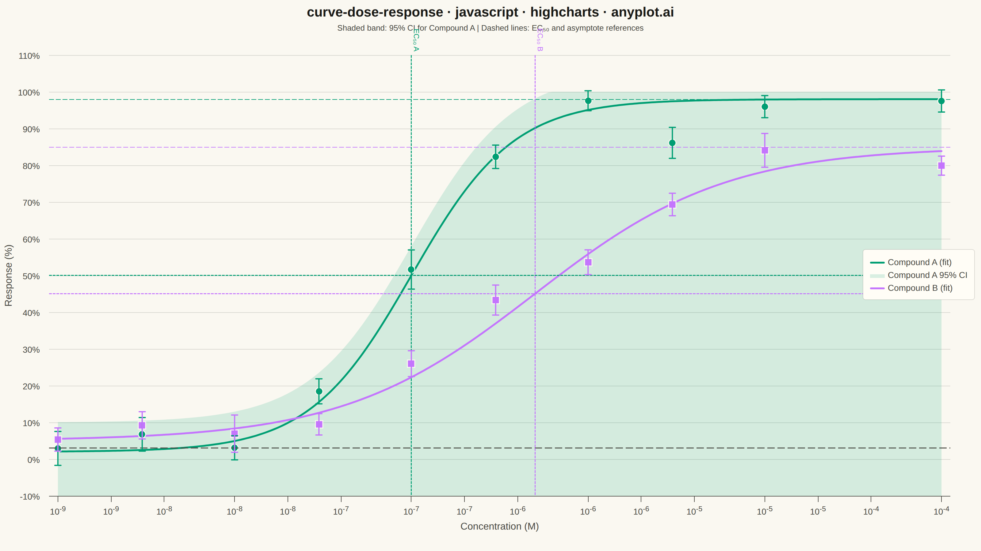
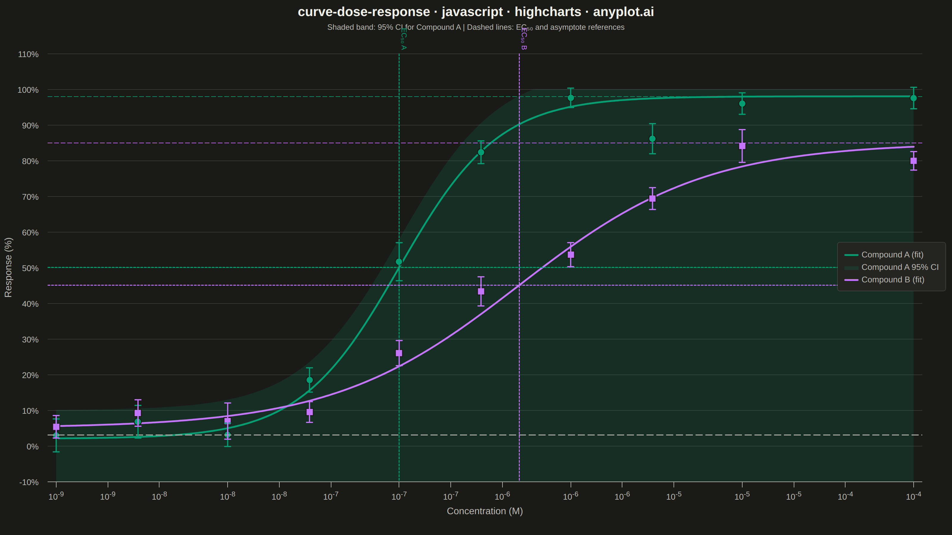
The same plot in 14 other libraries — JavaScript: Chart.js, D3.js, Apache ECharts, MUI X Charts; Python: Altair, Bokeh, lets-plot, Matplotlib, Plotly, plotnine, Pygal, Seaborn; R: ggplot2; Julia: Makie.jl. Compare all 15 side by side: Pharmacological Dose-Response Curve in Python, R, Julia and JavaScript.
A sigmoidal dose-response curve that plots biological response against drug concentration on a logarithmic x-axis, fitted using a four-parameter logistic (4PL) model. This visualization is essential for determining drug potency metrics such as EC50 (half-maximal effective concentration) or IC50 (half-maximal inhibitory concentration), Hill slope steepness, and upper/lower response asymptotes. It enables rapid visual comparison of compound efficacy and is a standard tool in pharmacological analysis.
// anyplot.ai
// curve-dose-response: Pharmacological Dose-Response Curve
// Library: highcharts 12.6.0 | JavaScript 22.22.3
// Quality: 87/100 | Created: 2026-06-24
//# anyplot-orientation: landscape

const t = window.ANYPLOT_TOKENS;

// --- Data --------------------------------------------------------------------

// 4-parameter logistic (4PL) sigmoid model
function fourPL(c, bottom, top, ec50, hill) {
    return bottom + (top - bottom) / (1 + Math.pow(ec50 / c, hill));
}

// Generate smooth fitted curve across 200 log-spaced points (1e-9 to 1e-4 M)
function smoothCurve(p) {
    const pts = [];
    for (let i = 0; i <= 200; i++) {
        const logC = -9 + 5 * i / 200;
        const c = Math.pow(10, logC);
        pts.push([c, fourPL(c, p.bottom, p.top, p.ec50, p.hill)]);
    }
    return pts;
}

// Deterministic LCG pseudo-random generator (reproducible, no seed API in browser)
function makeLCG(seed) {
    let s = seed >>> 0;
    return function () {
        s = (Math.imul(s, 1664525) + 1013904223) >>> 0;
        return s / 4294967296;
    };
}
function boxMuller(rng) {
    const u1 = rng() + 1e-10, u2 = rng();
    return Math.sqrt(-2 * Math.log(u1)) * Math.cos(2 * Math.PI * u2);
}

// Compound parameters — pharmacology drug-potency scenario
const compA = { name: 'Compound A', bottom: 2, top: 98, ec50: 1e-7, hill: 1.5 };
const compB = { name: 'Compound B', bottom: 5, top: 85, ec50: 5e-7, hill: 0.8 };

// Measurement concentrations: 10 log-spaced points from 1 nM to 100 µM
const measConc = [1e-9, 3e-9, 1e-8, 3e-8, 1e-7, 3e-7, 1e-6, 3e-6, 1e-5, 1e-4];

function genMeasured(p, seedVal) {
    const rng = makeLCG(seedVal);
    return measConc.map(c => {
        const ideal = fourPL(c, p.bottom, p.top, p.ec50, p.hill);
        const sem = 2.5 + Math.abs(boxMuller(rng)) * 1.5;
        const noise = boxMuller(rng) * sem;
        return { x: c, y: Math.max(0, Math.min(100, ideal + noise)), sem };
    });
}

const dataA = genMeasured(compA, 42);
const dataB = genMeasured(compB, 137);

const curveA = smoothCurve(compA);
const curveB = smoothCurve(compB);

// 95% CI band for Compound A: ±8 response units around fitted curve
const CI_W = 8;
const ciUpperA = curveA.map(([x, y]) => [x, Math.min(100, y + CI_W)]);

// Half-maximal response thresholds for EC50 reference lines
const halfA = (compA.bottom + compA.top) / 2;  // 50 %
const halfB = (compB.bottom + compB.top) / 2;  // 45 %

// RGBA for CI band: #009E73 = rgb(0,158,115) at 15% opacity
const ciColorA = 'rgba(0,158,115,0.15)';

// --- Chart -------------------------------------------------------------------

Highcharts.chart('container', {
    chart: {
        backgroundColor: 'transparent',
        animation: false,
        style: { fontFamily: 'inherit' },
        marginTop: 90,
        marginRight: 50,
        marginBottom: 90,
        marginLeft: 80,
        events: {
            // Draw error bars via SVG renderer after each render
            render: function () {
                const c = this;
                if (c._errorBars) c._errorBars.forEach(el => el.destroy());
                c._errorBars = [];

                // Series indices 3 (Compound A data) and 4 (Compound B data)
                [[3, t.palette[0]], [4, t.palette[1]]].forEach(([si, color]) => {
                    const s = c.series[si];
                    if (!s || !s.points) return;
                    s.points.forEach(pt => {
                        if (pt.plotX === undefined || pt.plotY === undefined) return;
                        const sem = (pt.options && pt.options.sem) || 3;
                        const px = pt.plotX + c.plotLeft;
                        const topY = c.yAxis[0].toPixels(pt.y + sem, false);
                        const botY = c.yAxis[0].toPixels(pt.y - sem, false);
                        const cap = 5;
                        const path = c.renderer.path([
                            'M', px, topY, 'L', px, botY,
                            'M', px - cap, topY, 'L', px + cap, topY,
                            'M', px - cap, botY, 'L', px + cap, botY
                        ]).attr({
                            stroke: color,
                            'stroke-width': 2,
                            zIndex: 10,
                            'stroke-linecap': 'round'
                        }).add();
                        c._errorBars.push(path);
                    });
                });
            }
        }
    },
    credits: { enabled: false },
    colors: t.palette,

    title: {
        text: 'curve-dose-response · javascript · highcharts · anyplot.ai',
        style: { color: t.ink, fontSize: '22px', fontWeight: '600' }
    },
    subtitle: {
        text: 'Shaded band: 95% CI for Compound A  |  Dashed lines: EC₅₀ and asymptote references',
        style: { color: t.inkSoft, fontSize: '13px' }
    },

    xAxis: {
        type: 'logarithmic',
        title: {
            text: 'Concentration (M)',
            style: { color: t.inkSoft, fontSize: '16px' }
        },
        lineColor: t.inkSoft,
        tickColor: t.inkSoft,
        gridLineColor: t.grid,
        gridLineWidth: 0,
        labels: {
            style: { color: t.inkSoft, fontSize: '14px' },
            formatter: function () {
                const exp = Math.round(Math.log10(this.value));
                return '10<sup>' + exp + '</sup>';
            },
            useHTML: true
        },
        plotLines: [
            {
                value: compA.ec50,
                color: t.palette[0],
                dashStyle: 'ShortDash',
                width: 1.5,
                zIndex: 5,
                label: {
                    text: 'EC₅₀ A',
                    style: { color: t.palette[0], fontSize: '12px' },
                    align: 'right',
                    y: -6
                }
            },
            {
                value: compB.ec50,
                color: t.palette[1],
                dashStyle: 'ShortDash',
                width: 1.5,
                zIndex: 5,
                label: {
                    text: 'EC₅₀ B',
                    style: { color: t.palette[1], fontSize: '12px' },
                    align: 'right',
                    y: -6
                }
            }
        ]
    },

    yAxis: {
        title: {
            text: 'Response (%)',
            style: { color: t.inkSoft, fontSize: '16px' }
        },
        lineColor: t.inkSoft,
        tickColor: t.inkSoft,
        gridLineColor: t.grid,
        gridLineWidth: 1,
        labels: {
            style: { color: t.inkSoft, fontSize: '14px' },
            format: '{value}%'
        },
        min: -5,
        max: 110,
        plotLines: [
            // EC50 half-max horizontal reference lines
            { value: halfA, color: t.palette[0], dashStyle: 'ShortDash', width: 1.5, zIndex: 5 },
            { value: halfB, color: t.palette[1], dashStyle: 'ShortDash', width: 1.5, zIndex: 5 },
            // Top asymptotes
            { value: compA.top, color: t.palette[0], dashStyle: 'LongDash', width: 1, zIndex: 4 },
            { value: compB.top, color: t.palette[1], dashStyle: 'LongDash', width: 1, zIndex: 4 },
            // Bottom asymptote (shared)
            { value: 3, color: t.inkSoft, dashStyle: 'LongDash', width: 1.5, zIndex: 4 }
        ]
    },

    legend: {
        enabled: true,
        align: 'right',
        verticalAlign: 'middle',
        layout: 'vertical',
        itemStyle: { color: t.inkSoft, fontSize: '14px' },
        itemHoverStyle: { color: t.ink },
        backgroundColor: t.elevatedBg,
        borderColor: t.grid,
        borderWidth: 1,
        borderRadius: 4,
        padding: 12,
        symbolWidth: 24
    },

    plotOptions: {
        series: { animation: false },
        spline: {
            lineWidth: 3,
            marker: { enabled: false }
        },
        scatter: {
            marker: { radius: 6 }
        }
    },

    series: [
        // Compound A fitted curve (show first so it appears first in legend)
        {
            type: 'spline',
            id: 'curveA',
            name: 'Compound A (fit)',
            data: curveA,
            color: t.palette[0],
            lineWidth: 3,
            zIndex: 5,
            showInLegend: true
        },
        // Compound A 95% CI band — upper envelope fill
        {
            type: 'area',
            name: 'Compound A 95% CI',
            data: ciUpperA,
            color: t.palette[0],
            fillColor: ciColorA,
            lineWidth: 0,
            threshold: null,
            showInLegend: true,
            enableMouseTracking: false,
            marker: { enabled: false },
            zIndex: 1
        },
        // Compound B fitted curve
        {
            type: 'spline',
            id: 'curveB',
            name: 'Compound B (fit)',
            data: curveB,
            color: t.palette[1],
            lineWidth: 3,
            zIndex: 5,
            showInLegend: true
        },
        // Compound A measured data points (linked to curveA for legend toggling)
        {
            type: 'scatter',
            name: 'Compound A (data)',
            data: dataA.map(d => ({ x: d.x, y: d.y, sem: d.sem })),
            color: t.palette[0],
            marker: {
                radius: 6,
                symbol: 'circle',
                lineWidth: 1.5,
                lineColor: t.pageBg
            },
            zIndex: 8,
            linkedTo: 'curveA',
            showInLegend: false,
            enableMouseTracking: false
        },
        // Compound B measured data points (linked to curveB for legend toggling)
        {
            type: 'scatter',
            name: 'Compound B (data)',
            data: dataB.map(d => ({ x: d.x, y: d.y, sem: d.sem })),
            color: t.palette[1],
            marker: {
                radius: 6,
                symbol: 'square',
                lineWidth: 1.5,
                lineColor: t.pageBg
            },
            zIndex: 8,
            linkedTo: 'curveB',
            showInLegend: false,
            enableMouseTracking: false
        }
    ]
});
Runnable source as JSON, for any HTTP client: https://api.anyplot.ai/specs/curve-dose-response/highcharts/code. Any spec id and library id listed in llms-full.txt fit the same URL shape; every URL below is complete and callable.
{
  "spec_id": "curve-dose-response",
  "language": "javascript",
  "library": "highcharts",
  "page": "https://anyplot.ai/curve-dose-response/javascript/highcharts",
  "hub": "https://anyplot.ai/curve-dose-response",
  "code_json": "https://api.anyplot.ai/specs/curve-dose-response/highcharts/code",
  "spec_json": "https://api.anyplot.ai/specs/curve-dose-response",
  "render_light_png": "https://storage.googleapis.com/anyplot-images/plots/curve-dose-response/javascript/highcharts/plot-light.png",
  "render_dark_png": "https://storage.googleapis.com/anyplot-images/plots/curve-dose-response/javascript/highcharts/plot-dark.png",
  "interactive_light_html": "https://storage.googleapis.com/anyplot-images/plots/curve-dose-response/javascript/highcharts/plot-light.html",
  "interactive_dark_html": "https://storage.googleapis.com/anyplot-images/plots/curve-dose-response/javascript/highcharts/plot-dark.html",
  "quality_score": 87.0,
  "license": "MIT",
  "guide": "https://anyplot.ai/llms.txt"
}
Part of Pharmacological Dose-Response Curve on anyplot.ai.