The same plot in 14 other libraries — JavaScript: Chart.js, D3.js, Highcharts, MUI X Charts; Python: Altair, Bokeh, lets-plot, Matplotlib, Plotly, plotnine, Pygal, Seaborn; R: ggplot2; Julia: Makie.jl. Compare all 15 side by side: Pharmacological Dose-Response Curve in Python, R, Julia and JavaScript.
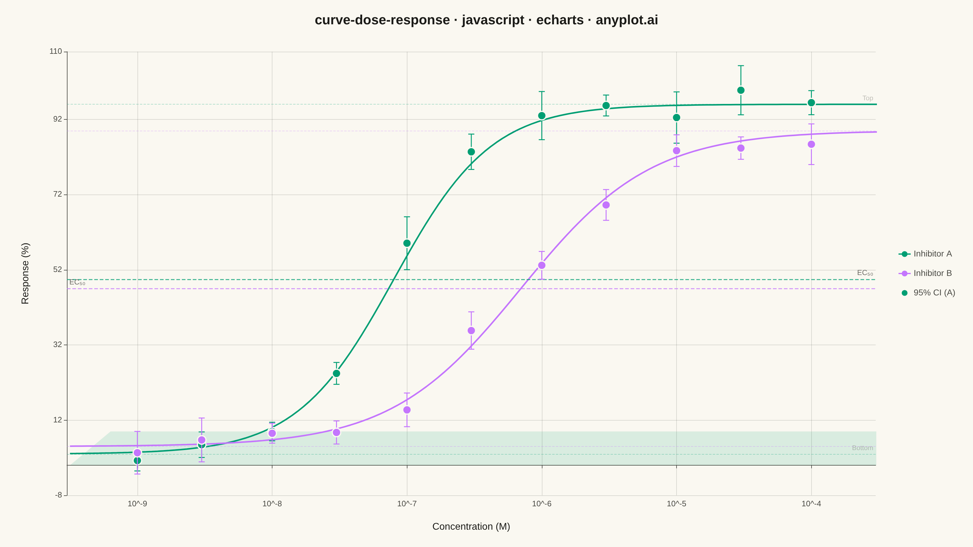
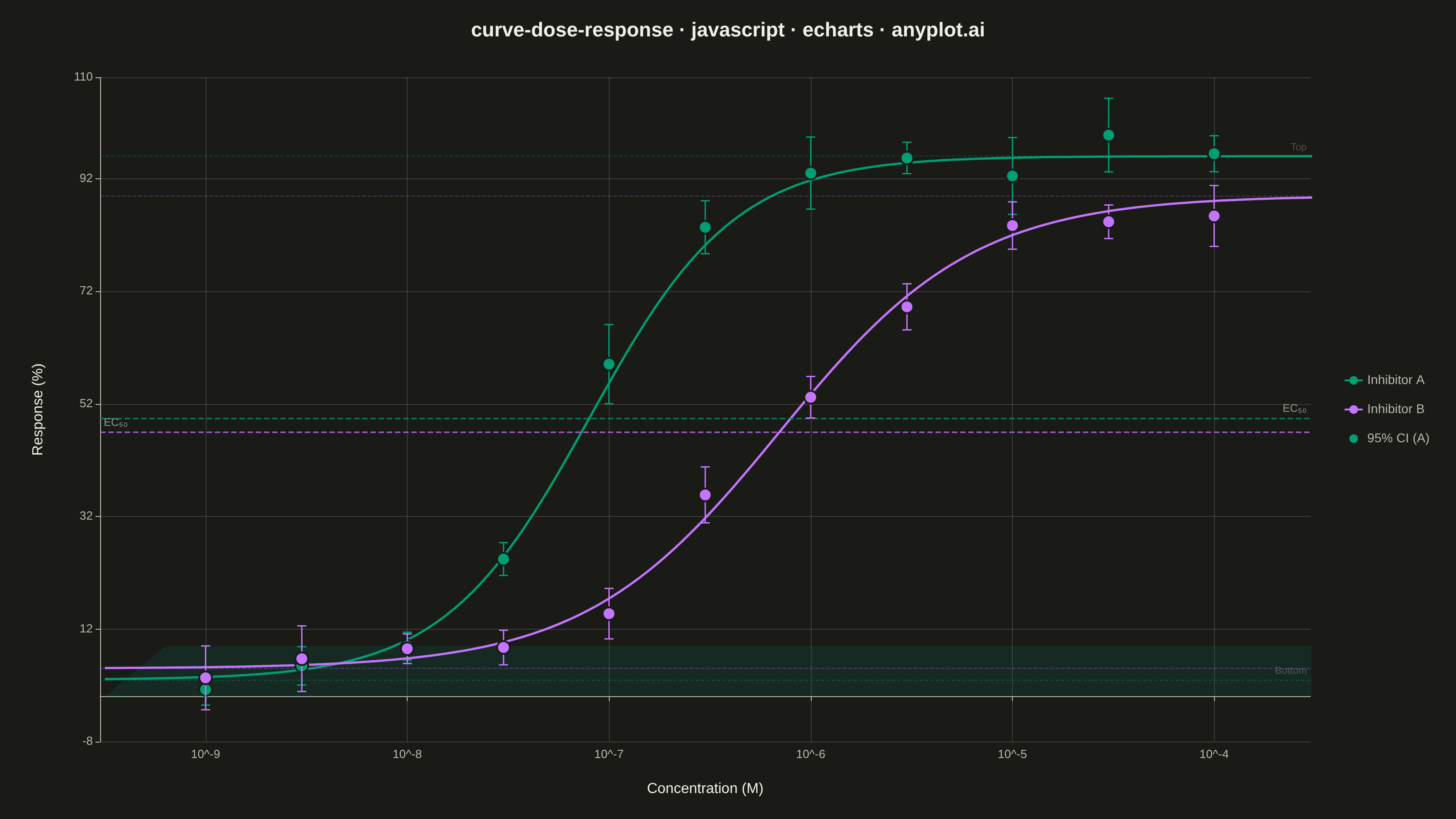
A sigmoidal dose-response curve that plots biological response against drug concentration on a logarithmic x-axis, fitted using a four-parameter logistic (4PL) model. This visualization is essential for determining drug potency metrics such as EC50 (half-maximal effective concentration) or IC50 (half-maximal inhibitory concentration), Hill slope steepness, and upper/lower response asymptotes. It enables rapid visual comparison of compound efficacy and is a standard tool in pharmacological analysis.
// anyplot.ai
// curve-dose-response: Pharmacological Dose-Response Curve
// Library: echarts 5.5.1 | JavaScript 22.23.0
// Quality: 90/100 | Created: 2026-06-24

const t = window.ANYPLOT_TOKENS;

// 4-parameter logistic (4PL) model
function pl4(c, bot, top, ec50, hill) {
  return bot + (top - bot) / (1 + Math.pow(ec50 / c, hill));
}

// Deterministic LCG RNG
let _s = 0;
function srand(n) { _s = n >>> 0; }
function rand() {
  _s = (_s * 1664525 + 1013904223) & 0xffffffff;
  return (_s >>> 0) / 4294967295;
}

// Kinase inhibitor study: two compounds with different potencies
const cmpA = { name: 'Inhibitor A', bot: 3,  top: 96, ec50: 8e-8, hill: 1.2 };
const cmpB = { name: 'Inhibitor B', bot: 5,  top: 89, ec50: 7e-7, hill: 0.9 };

// Experimental concentration points (log-spaced, 1 nM – 100 µM)
const concs = [1e-9, 3e-9, 1e-8, 3e-8, 1e-7, 3e-7, 1e-6, 3e-6, 1e-5, 3e-5, 1e-4];

function makeExpData(cmp, seed) {
  srand(seed);
  return concs.map(c => [
    c,
    Math.max(0, Math.min(100, pl4(c, cmp.bot, cmp.top, cmp.ec50, cmp.hill) + (rand() - 0.5) * 9)),
    1.2 + rand() * 2.4,
  ]);
}

const expA = makeExpData(cmpA, 42);
const expB = makeExpData(cmpB, 137);

// Smooth fitted curves (150 log-spaced evaluation points)
const xCurve = Array.from({ length: 151 }, (_, i) => Math.pow(10, -9.5 + i * 6.5 / 150));
const curveA = xCurve.map(c => [c, pl4(c, cmpA.bot, cmpA.top, cmpA.ec50, cmpA.hill)]);
const curveB = xCurve.map(c => [c, pl4(c, cmpB.bot, cmpB.top, cmpB.ec50, cmpB.hill)]);

// 95% CI band around Inhibitor A (±4.5 response units, stacked area technique)
const CI = 4.5;
const ciLow  = xCurve.map(c => [c, pl4(c, cmpA.bot, cmpA.top, cmpA.ec50, cmpA.hill) - CI]);
const ciDiff = xCurve.map(c => [c, CI * 2]);

// EC50 half-maximal response (midpoint of 4PL = (bot + top) / 2)
const midA = (cmpA.bot + cmpA.top) / 2;
const midB = (cmpB.bot + cmpB.top) / 2;

// Custom renderItem for scatter points with ±1.96 SEM error bars
function makeEBSeries(data, color, name) {
  return {
    type: 'custom',
    name,
    legendHoverLink: false,
    renderItem(_params, api) {
      const [px, py]  = api.coord([api.value(0), api.value(1)]);
      const [, ytop]  = api.coord([api.value(0), api.value(1) + api.value(2) * 1.96]);
      const [, ybot]  = api.coord([api.value(0), api.value(1) - api.value(2) * 1.96]);
      const cap = 5;
      return {
        type: 'group',
        children: [
          { type: 'line', shape: { x1: px, y1: ytop, x2: px, y2: ybot },
            style: { stroke: color, lineWidth: 1.5 } },
          { type: 'line', shape: { x1: px - cap, y1: ytop, x2: px + cap, y2: ytop },
            style: { stroke: color, lineWidth: 1.5 } },
          { type: 'line', shape: { x1: px - cap, y1: ybot, x2: px + cap, y2: ybot },
            style: { stroke: color, lineWidth: 1.5 } },
          { type: 'circle', shape: { cx: px, cy: py, r: 7 },
            style: { fill: color, stroke: t.pageBg, lineWidth: 2 } },
        ],
      };
    },
    data,
    z: 10,
  };
}

const chart = echarts.init(document.getElementById('container'));

chart.setOption({
  animation: false,
  backgroundColor: 'transparent',
  color: t.palette,

  title: {
    text: 'curve-dose-response · javascript · echarts · anyplot.ai',
    left: 'center',
    top: 18,
    textStyle: { color: t.ink, fontSize: 22, fontWeight: 'bold' },
  },

  legend: {
    data: [cmpA.name, cmpB.name, '95% CI (A)'],
    orient: 'vertical',
    right: 24,
    top: 'middle',
    textStyle: { color: t.inkSoft, fontSize: 14 },
    itemGap: 18,
    itemWidth: 20,
    itemHeight: 12,
  },

  grid: { left: 110, right: 160, top: 85, bottom: 85 },

  xAxis: {
    type: 'log',
    name: 'Concentration (M)',
    nameLocation: 'middle',
    nameGap: 44,
    nameTextStyle: { color: t.ink, fontSize: 16 },
    min: 3e-10,
    max: 3e-4,
    axisLabel: {
      color: t.inkSoft,
      fontSize: 13,
      formatter(v) {
        const logV = Math.log10(v);
        const e = Math.round(logV);
        return Math.abs(logV - e) < 0.01 ? '10^' + e : '';
      },
    },
    axisLine: { lineStyle: { color: t.inkSoft } },
    splitLine: { lineStyle: { color: t.grid } },
    minorSplitLine: { show: true, lineStyle: { color: t.grid, opacity: 0.45 } },
    minorTick: { show: true },
  },

  yAxis: {
    type: 'value',
    name: 'Response (%)',
    nameLocation: 'middle',
    nameGap: 60,
    nameTextStyle: { color: t.ink, fontSize: 16 },
    min: -8,
    max: 110,
    interval: 20,
    axisLabel: { color: t.inkSoft, fontSize: 13 },
    axisLine: { lineStyle: { color: t.inkSoft } },
    splitLine: { lineStyle: { color: t.grid } },
  },

  series: [
    // CI band lower boundary (invisible baseline for stacking)
    {
      type: 'line',
      name: '_ci_base',
      data: ciLow,
      lineStyle: { opacity: 0 },
      areaStyle: { opacity: 0 },
      stack: 'ci-a',
      symbol: 'none',
      silent: true,
    },
    // CI band upper (stacked on base — fills the band between lower and upper)
    {
      type: 'line',
      name: '95% CI (A)',
      data: ciDiff,
      lineStyle: { opacity: 0 },
      areaStyle: { color: t.palette[0], opacity: 0.13 },
      stack: 'ci-a',
      symbol: 'none',
      color: t.palette[0],
      silent: true,
    },

    // Fitted curve — Inhibitor A with EC50 + asymptote reference lines
    {
      type: 'line',
      name: cmpA.name,
      data: curveA,
      smooth: false,
      symbol: 'none',
      lineStyle: { color: t.palette[0], width: 2.5 },
      color: t.palette[0],
      markLine: {
        silent: true,
        symbol: 'none',
        label: { show: false },
        data: [
          {
            yAxis: midA,
            lineStyle: { color: t.palette[0], type: 'dashed', opacity: 0.8, width: 1.5 },
            label: { show: true, formatter: 'EC₅₀', position: 'insideEndTop',
                     color: t.inkSoft, fontSize: 12, distance: [4, 4] },
          },
          {
            xAxis: cmpA.ec50,
            lineStyle: { color: t.palette[0], type: 'dashed', opacity: 0.8, width: 1.5 },
          },
          {
            yAxis: cmpA.top,
            lineStyle: { color: t.palette[0], type: 'dashed', opacity: 0.32, width: 1 },
            label: { show: true, formatter: 'Top', position: 'insideEndTop',
                     color: t.inkSoft, fontSize: 11, distance: [4, 4] },
          },
          {
            yAxis: cmpA.bot,
            lineStyle: { color: t.palette[0], type: 'dashed', opacity: 0.32, width: 1 },
            label: { show: true, formatter: 'Bottom', position: 'insideEndTop',
                     color: t.inkSoft, fontSize: 11, distance: [4, 4] },
          },
        ],
      },
    },

    // Fitted curve — Inhibitor B with EC50 + asymptote reference lines
    {
      type: 'line',
      name: cmpB.name,
      data: curveB,
      smooth: false,
      symbol: 'none',
      lineStyle: { color: t.palette[1], width: 2.5 },
      color: t.palette[1],
      markLine: {
        silent: true,
        symbol: 'none',
        label: { show: false },
        data: [
          {
            yAxis: midB,
            lineStyle: { color: t.palette[1], type: 'dashed', opacity: 0.8, width: 1.5 },
            label: { show: true, formatter: 'EC₅₀', position: 'insideStartTop',
                     color: t.inkSoft, fontSize: 12, distance: [4, 4] },
          },
          {
            xAxis: cmpB.ec50,
            lineStyle: { color: t.palette[1], type: 'dashed', opacity: 0.8, width: 1.5 },
          },
          {
            yAxis: cmpB.top,
            lineStyle: { color: t.palette[1], type: 'dashed', opacity: 0.32, width: 1 },
          },
          {
            yAxis: cmpB.bot,
            lineStyle: { color: t.palette[1], type: 'dashed', opacity: 0.32, width: 1 },
          },
        ],
      },
    },

    // Scatter + error bars for Inhibitor A
    makeEBSeries(expA, t.palette[0], '_eb_a'),
    // Scatter + error bars for Inhibitor B
    makeEBSeries(expB, t.palette[1], '_eb_b'),
  ],
});
Runnable source as JSON, for any HTTP client: https://api.anyplot.ai/specs/curve-dose-response/echarts/code. Any spec id and library id listed in llms-full.txt fit the same URL shape; every URL below is complete and callable.
{
  "spec_id": "curve-dose-response",
  "language": "javascript",
  "library": "echarts",
  "page": "https://anyplot.ai/curve-dose-response/javascript/echarts",
  "hub": "https://anyplot.ai/curve-dose-response",
  "code_json": "https://api.anyplot.ai/specs/curve-dose-response/echarts/code",
  "spec_json": "https://api.anyplot.ai/specs/curve-dose-response",
  "render_light_png": "https://storage.googleapis.com/anyplot-images/plots/curve-dose-response/javascript/echarts/plot-light.png",
  "render_dark_png": "https://storage.googleapis.com/anyplot-images/plots/curve-dose-response/javascript/echarts/plot-dark.png",
  "interactive_light_html": "https://storage.googleapis.com/anyplot-images/plots/curve-dose-response/javascript/echarts/plot-light.html",
  "interactive_dark_html": "https://storage.googleapis.com/anyplot-images/plots/curve-dose-response/javascript/echarts/plot-dark.html",
  "quality_score": 90.0,
  "license": "MIT",
  "guide": "https://anyplot.ai/llms.txt"
}
Part of Pharmacological Dose-Response Curve on anyplot.ai.