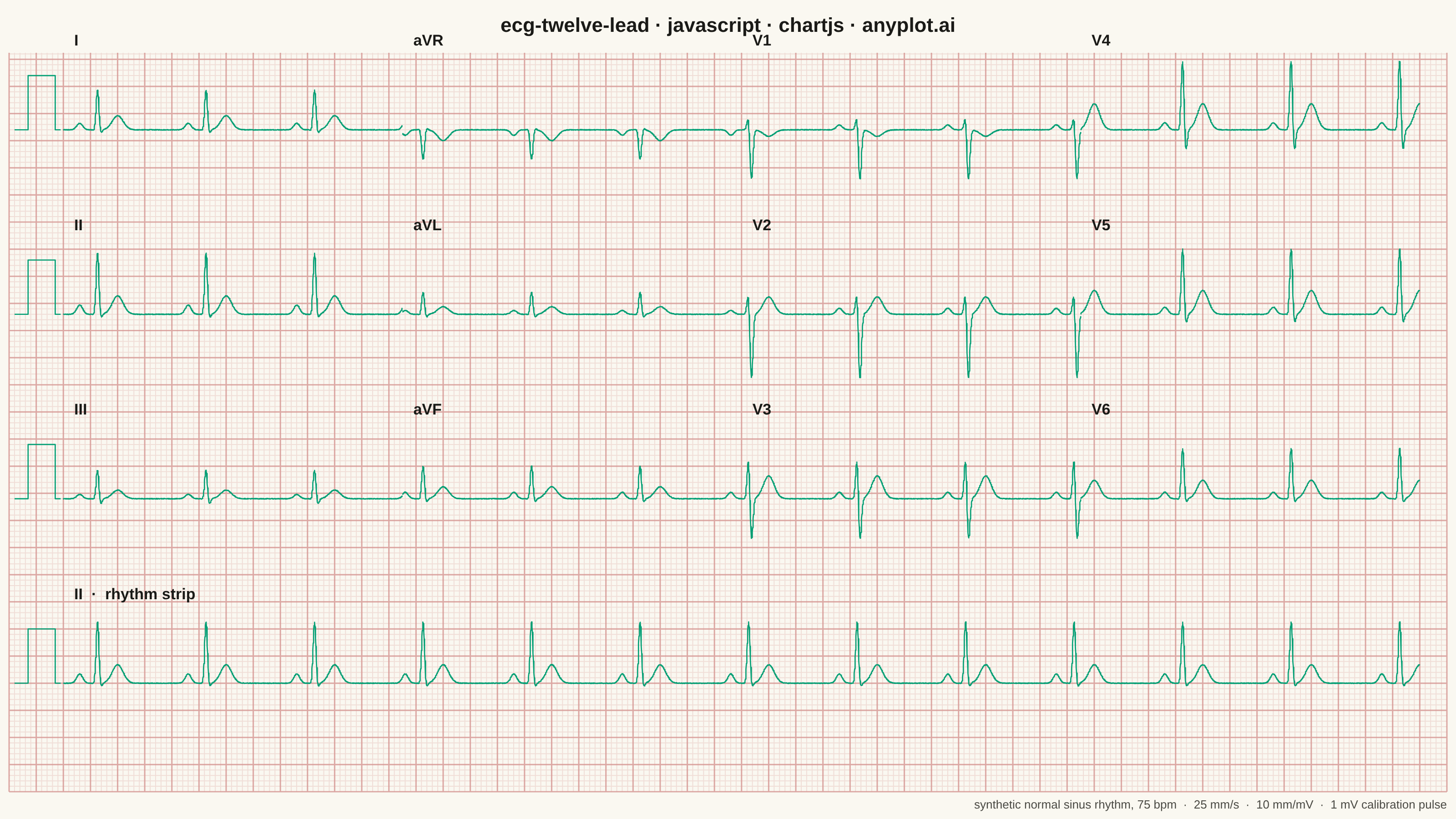
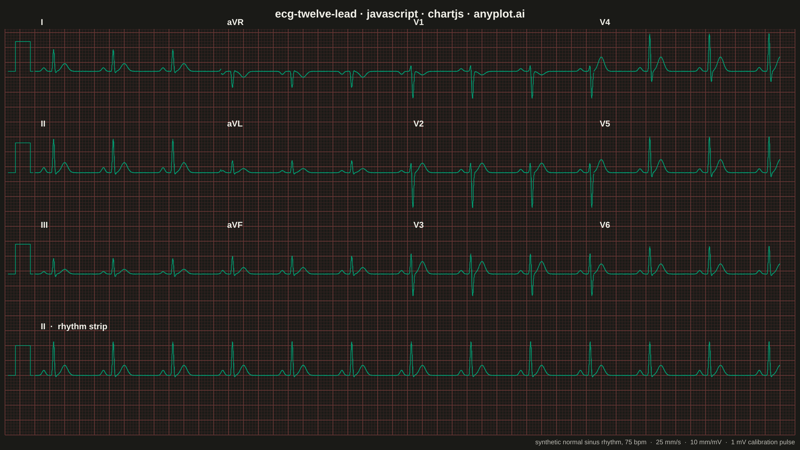
A multi-channel electrocardiogram display showing the 12 standard ECG leads arranged in clinical format. Each lead displays realistic P-QRS-T wave complexes on a medical-standard grid background with calibration markers. This visualization replicates the familiar layout used in hospitals and clinics worldwide, making it immediately recognizable to healthcare professionals and useful for medical education.
// anyplot.ai
// ecg-twelve-lead: ECG/EKG 12-Lead Waveform Display
// Library: chartjs 4.4.7 | JavaScript 22.22.3
// Quality: 93/100 | Created: 2026-06-17
//# anyplot-orientation: landscape

const t = window.ANYPLOT_TOKENS;
const TRACE = t.palette[0]; // #009E73 Imprint brand green — the single signal series

// Theme-adaptive ECG "paper" grid (light red / pink), drawn over the warm
// page background instead of pure white so it stays on the Imprint surface.
const isDark = window.ANYPLOT_THEME === "dark";
const GRID_MINOR = isDark ? "rgba(199,90,90,0.16)" : "rgba(174,48,48,0.13)";
const GRID_MAJOR = isDark ? "rgba(199,90,90,0.34)" : "rgba(174,48,48,0.32)";

// --- Synthetic 12-lead signal (normal sinus rhythm, ~75 bpm) ----------------
// Each lead is a sum of Gaussian P-Q-R-S-T deflections (mV); per-lead amplitudes
// encode the normal cardiac axis (aVR inverted, V1 rS → V6 qR progression).
const LEADS = {
  I:   { p: 0.12, q: -0.04, r: 0.75, s: -0.10, t: 0.26 },
  II:  { p: 0.17, q: -0.04, r: 1.15, s: -0.12, t: 0.34 },
  III: { p: 0.08, q: -0.03, r: 0.55, s: -0.14, t: 0.16 },
  aVR: { p: -0.10, q: 0.03, r: -0.55, s: 0.05, t: -0.20 },
  aVL: { p: 0.07, q: -0.03, r: 0.42, s: -0.08, t: 0.14 },
  aVF: { p: 0.12, q: -0.03, r: 0.62, s: -0.10, t: 0.22 },
  V1:  { p: 0.09, q: 0.0, r: 0.28, s: -0.95, t: -0.12 },
  V2:  { p: 0.11, q: 0.0, r: 0.45, s: -1.25, t: 0.32 },
  V3:  { p: 0.12, q: -0.02, r: 0.80, s: -0.85, t: 0.42 },
  V4:  { p: 0.13, q: -0.04, r: 1.35, s: -0.50, t: 0.48 },
  V5:  { p: 0.13, q: -0.05, r: 1.25, s: -0.25, t: 0.44 },
  V6:  { p: 0.12, q: -0.05, r: 0.95, s: -0.12, t: 0.34 },
};

// Deterministic tiny baseline noise (fixed-seed LCG — no Math.random in harness).
let seed = 12345;
const noise = () => {
  seed = (1103515245 * seed + 12345) % 2147483648;
  return (seed / 2147483648 - 0.5) * 0.012;
};

const BEAT = 0.8; // seconds per cardiac cycle → 75 bpm
const gauss = (ph, mu, sig) => Math.exp(-((ph - mu) * (ph - mu)) / (2 * sig * sig));
function voltage(cfg, time) {
  const ph = time % BEAT;
  return (
    cfg.p * gauss(ph, 0.12, 0.022) +
    cfg.q * gauss(ph, 0.232, 0.0085) +
    cfg.r * gauss(ph, 0.252, 0.011) +
    cfg.s * gauss(ph, 0.272, 0.011) +
    cfg.t * gauss(ph, 0.40, 0.040) +
    noise()
  );
}

// --- Layout geometry (millimetre paper space; 25 mm/s, 10 mm/mV) ------------
// Standard clinical 3×4 grid + a full-length Lead II rhythm strip beneath it.
const GRID = [
  ["I", "aVR", "V1", "V4"],
  ["II", "aVL", "V2", "V5"],
  ["III", "aVF", "V3", "V6"],
];
const LEFT = 10;        // left margin (holds the calibration pulse)
const STRIP_MM = 62.5;  // 2.5 s column at 25 mm/s
const MM_PER_S = 25;
const MM_PER_MV = 10;
const ROW_Y = [122, 88, 54]; // baselines, top → bottom
const RHYTHM_Y = 20;
const X_MAX = LEFT + 4 * STRIP_MM + 5; // 265
const Y_MAX = 136.2; // tuned so 1 mm paper squares stay square at 16:9
const DT = 0.002;

// One cell of the grid: a 2.5 s window of the continuous recording.
function cellTrace(lead, col, baseline) {
  const cfg = LEADS[lead];
  const t0 = 2.5 * col;
  const pts = [];
  for (let time = t0; time <= t0 + 2.5 + 1e-9; time += DT) {
    pts.push({ x: LEFT + col * STRIP_MM + (time - t0) * MM_PER_S, y: baseline + voltage(cfg, time) * MM_PER_MV });
  }
  return pts;
}

const datasets = [];
GRID.forEach((row, r) =>
  row.forEach((lead, c) => datasets.push({ data: cellTrace(lead, c, ROW_Y[r]) }))
);

// Full 10 s Lead II rhythm strip across the bottom.
const rhythm = [];
for (let time = 0; time <= 10 + 1e-9; time += DT) {
  rhythm.push({ x: LEFT + time * MM_PER_S, y: RHYTHM_Y + voltage(LEADS.II, time) * MM_PER_MV });
}
datasets.push({ data: rhythm });

// 1 mV calibration pulse at the left margin of every row.
const calPulse = (b) => [
  { x: 1, y: b }, { x: 3.5, y: b }, { x: 3.5, y: b + 10 },
  { x: 8.5, y: b + 10 }, { x: 8.5, y: b }, { x: 9.5, y: b },
];
[...ROW_Y, RHYTHM_Y].forEach((b) => datasets.push({ data: calPulse(b) }));

// Shared trace styling — thin crisp green pen, no markers.
datasets.forEach((d) => {
  d.borderColor = TRACE;
  d.borderWidth = 1.3;
  d.pointRadius = 0;
  d.tension = 0;
  d.fill = false;
  d.borderJoinStyle = "round";
});

// --- ECG paper, lead labels, title (custom plugins) -------------------------
const ecgPaper = {
  id: "ecgPaper",
  beforeDatasetsDraw(chart) {
    const { ctx } = chart;
    const xs = chart.scales.x;
    const ys = chart.scales.y;
    const px = (v) => xs.getPixelForValue(v);
    const py = (v) => ys.getPixelForValue(v);

    const drawLines = (step, width, color) => {
      ctx.save();
      ctx.lineWidth = width;
      ctx.strokeStyle = color;
      ctx.beginPath();
      for (let x = 0; x <= X_MAX + 1e-6; x += step) {
        ctx.moveTo(px(x), py(0));
        ctx.lineTo(px(x), py(Y_MAX));
      }
      for (let y = 0; y <= Y_MAX + 1e-6; y += step) {
        ctx.moveTo(px(0), py(y));
        ctx.lineTo(px(X_MAX), py(y));
      }
      ctx.stroke();
      ctx.restore();
    };
    drawLines(1, 1, GRID_MINOR);
    drawLines(5, 1.6, GRID_MAJOR);
  },
  afterDatasetsDraw(chart) {
    const { ctx, chartArea: a } = chart;
    const xs = chart.scales.x;
    const ys = chart.scales.y;
    const px = (v) => xs.getPixelForValue(v);
    const py = (v) => ys.getPixelForValue(v);

    // Lead labels, anchored top-left of each cell.
    ctx.save();
    ctx.fillStyle = t.ink;
    ctx.font = "bold 17px -apple-system, BlinkMacSystemFont, 'Segoe UI', Roboto, sans-serif";
    ctx.textAlign = "left";
    ctx.textBaseline = "alphabetic";
    GRID.forEach((row, r) =>
      row.forEach((lead, c) => ctx.fillText(lead, px(LEFT + c * STRIP_MM + 2), py(ROW_Y[r] + 15.5)))
    );
    ctx.fillText("II  ·  rhythm strip", px(LEFT + 2), py(RHYTHM_Y + 15.5));
    ctx.restore();

    // Title in the reserved top band.
    ctx.save();
    ctx.fillStyle = t.ink;
    ctx.textAlign = "center";
    ctx.textBaseline = "middle";
    ctx.font = "bold 22px -apple-system, BlinkMacSystemFont, 'Segoe UI', Roboto, sans-serif";
    ctx.fillText("ecg-twelve-lead · javascript · chartjs · anyplot.ai", (a.left + a.right) / 2, a.top / 2);
    ctx.restore();

    // Scale footnote in the reserved bottom band.
    ctx.save();
    ctx.fillStyle = t.inkSoft;
    ctx.textAlign = "right";
    ctx.textBaseline = "middle";
    ctx.font = "13px -apple-system, BlinkMacSystemFont, 'Segoe UI', Roboto, sans-serif";
    ctx.fillText(
      "synthetic normal sinus rhythm, 75 bpm  ·  25 mm/s  ·  10 mm/mV  ·  1 mV calibration pulse",
      a.right,
      a.bottom + (chart.height - a.bottom) / 2
    );
    ctx.restore();
  },
};

// --- Mount ------------------------------------------------------------------
const canvas = document.createElement("canvas");
document.getElementById("container").appendChild(canvas);

new Chart(canvas, {
  type: "line",
  data: { datasets },
  options: {
    responsive: true,
    maintainAspectRatio: false,
    animation: false,
    parsing: false,
    layout: { padding: { left: 10, right: 10, top: 58, bottom: 30 } },
    plugins: {
      legend: { display: false },
      title: { display: false },
      tooltip: { enabled: false },
    },
    scales: {
      x: { type: "linear", min: 0, max: X_MAX, display: false },
      y: { type: "linear", min: 0, max: Y_MAX, display: false },
    },
  },
  plugins: [ecgPaper],
});
Runnable source as JSON, for any HTTP client: https://api.anyplot.ai/specs/ecg-twelve-lead/chartjs/code. Any spec id and library id listed in llms-full.txt fit the same URL shape; every URL below is complete and callable.
{
  "spec_id": "ecg-twelve-lead",
  "language": "javascript",
  "library": "chartjs",
  "page": "https://anyplot.ai/ecg-twelve-lead/javascript/chartjs",
  "hub": "https://anyplot.ai/ecg-twelve-lead",
  "code_json": "https://api.anyplot.ai/specs/ecg-twelve-lead/chartjs/code",
  "spec_json": "https://api.anyplot.ai/specs/ecg-twelve-lead",
  "render_light_png": "https://storage.googleapis.com/anyplot-images/plots/ecg-twelve-lead/javascript/chartjs/plot-light.png",
  "render_dark_png": "https://storage.googleapis.com/anyplot-images/plots/ecg-twelve-lead/javascript/chartjs/plot-dark.png",
  "interactive_light_html": "https://storage.googleapis.com/anyplot-images/plots/ecg-twelve-lead/javascript/chartjs/plot-light.html",
  "interactive_dark_html": "https://storage.googleapis.com/anyplot-images/plots/ecg-twelve-lead/javascript/chartjs/plot-dark.html",
  "quality_score": 93.0,
  "license": "MIT",
  "guide": "https://anyplot.ai/llms.txt"
}
Part of ECG/EKG 12-Lead Waveform Display on anyplot.ai.