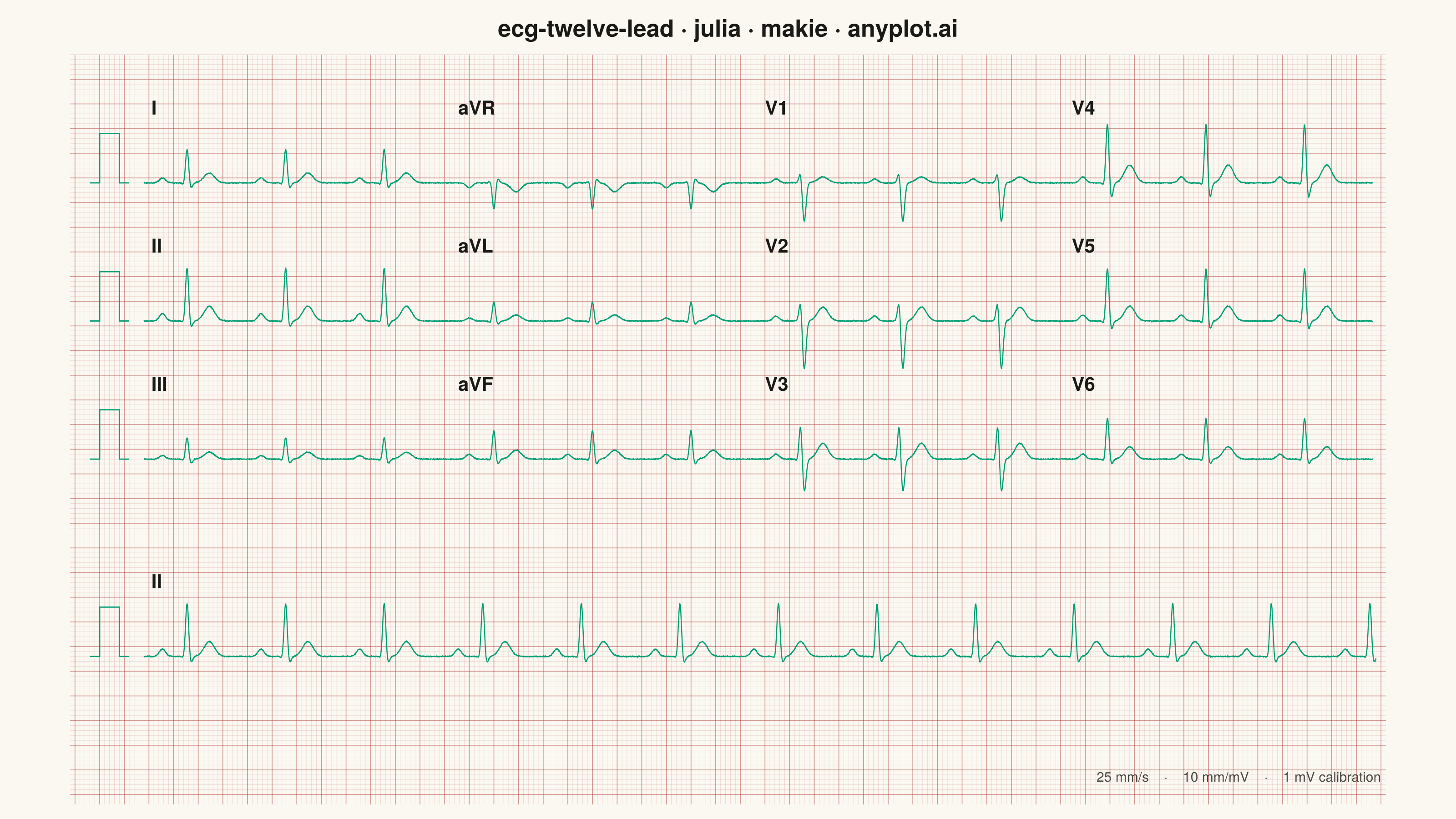
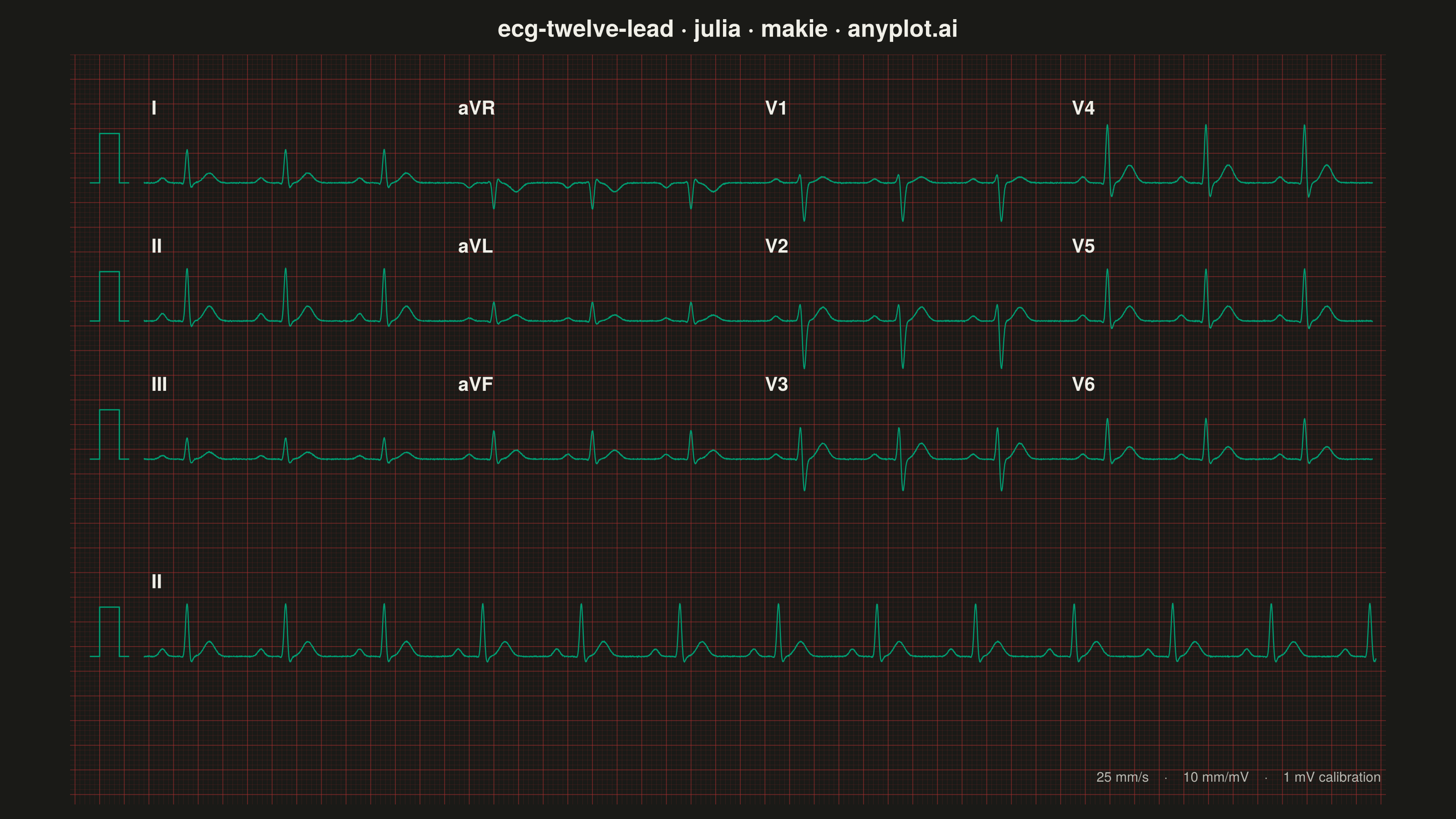
A multi-channel electrocardiogram display showing the 12 standard ECG leads arranged in clinical format. Each lead displays realistic P-QRS-T wave complexes on a medical-standard grid background with calibration markers. This visualization replicates the familiar layout used in hospitals and clinics worldwide, making it immediately recognizable to healthcare professionals and useful for medical education.
# anyplot.ai
# ecg-twelve-lead: ECG/EKG 12-Lead Waveform Display
# Library: makie 0.22.10 | Julia 1.11.9
# Quality: 93/100 | Created: 2026-06-17

using CairoMakie
using Colors
using Random

Random.seed!(42)

# --- Theme tokens -----------------------------------------------------------
const THEME    = get(ENV, "ANYPLOT_THEME", "light")
const PAGE_BG  = THEME == "light" ? colorant"#FAF8F1" : colorant"#1A1A17"
const INK      = THEME == "light" ? colorant"#1A1A17" : colorant"#F0EFE8"
const INK_SOFT = THEME == "light" ? colorant"#4A4A44" : colorant"#B8B7B0"

# Imprint palette position 1 (brand green) is the ECG trace — the first series.
const TRACE    = colorant"#009E73"
# Imprint matte red (#AE3030) renders the classic ECG paper grid; the theme
# background stays #FAF8F1 / #1A1A17 per the style guide.
const GRID_RED   = colorant"#AE3030"
const MINOR_A    = THEME == "light" ? 0.18 : 0.24
const MAJOR_A    = THEME == "light" ? 0.42 : 0.50
const GRID_MINOR = RGBAf(GRID_RED.r, GRID_RED.g, GRID_RED.b, MINOR_A)
const GRID_MAJOR = RGBAf(GRID_RED.r, GRID_RED.g, GRID_RED.b, MAJOR_A)

# --- Synthetic ECG model ----------------------------------------------------
# One P-QRS-T complex as a sum of Gaussians, in mV, centred on the R peak.
gauss(t, a, mu, sig) = a * exp(-((t - mu)^2) / (2 * sig^2))

beat(t, p) =
    gauss(t, p.P, -0.200, 0.025) +
    gauss(t, p.Q, -0.025, 0.012) +
    gauss(t, p.R,  0.000, 0.013) +
    gauss(t, p.S,  0.028, 0.015) +
    gauss(t, p.T,  0.180, 0.042)

# Per-lead morphology — normal sinus rhythm with standard polarities and the
# precordial R/S progression (deep S in V1/V2 → tall R in V4–V6); aVR inverted.
const LEAD_PARAMS = Dict(
    "I"   => (P =  0.10, Q = -0.05, R =  0.70, S = -0.12, T =  0.20),
    "II"  => (P =  0.15, Q = -0.05, R =  1.10, S = -0.15, T =  0.30),
    "III" => (P =  0.07, Q = -0.04, R =  0.45, S = -0.10, T =  0.14),
    "aVR" => (P = -0.10, Q =  0.05, R = -0.55, S =  0.10, T = -0.18),
    "aVL" => (P =  0.06, Q = -0.05, R =  0.40, S = -0.08, T =  0.12),
    "aVF" => (P =  0.10, Q = -0.04, R =  0.60, S = -0.12, T =  0.18),
    "V1"  => (P =  0.08, Q =  0.00, R =  0.25, S = -0.80, T =  0.12),
    "V2"  => (P =  0.10, Q =  0.00, R =  0.45, S = -1.00, T =  0.28),
    "V3"  => (P =  0.10, Q = -0.05, R =  0.75, S = -0.70, T =  0.32),
    "V4"  => (P =  0.12, Q = -0.08, R =  1.25, S = -0.35, T =  0.36),
    "V5"  => (P =  0.12, Q = -0.08, R =  1.10, S = -0.20, T =  0.30),
    "V6"  => (P =  0.10, Q = -0.06, R =  0.85, S = -0.12, T =  0.25),
)

# 1000 Hz sampling, ~75 bpm (RR = 0.80 s). Returns time (s) and voltage (mV).
function ecg_signal(duration, p; fs = 1000, rr = 0.80, first_r = 0.35)
    t = collect(0:1/fs:duration)
    v = zeros(length(t))
    for r0 in first_r:rr:duration
        v .+= beat.(t .- r0, Ref(p))
    end
    v .+= 0.006 .* randn(length(t))   # faint measurement noise
    return t, v
end

# --- Display geometry (millimetres: 25 mm/s horizontal, 10 mm/mV vertical) ---
const MM_PER_S  = 25.0
const MM_PER_MV = 10.0
const grid_layout = [
    ("I", "aVR", "V1", "V4"),
    ("II", "aVL", "V2", "V5"),
    ("III", "aVF", "V3", "V6"),
]
const row_centers = [124.0, 96.0, 68.0]            # top → bottom
const col_starts  = [14.0, 76.25, 138.5, 200.75]   # 2.5 s (62.5 mm) per column
const X_MAX = 265.0
const Y_MAX = 150.0

# --- Figure -----------------------------------------------------------------
fig = Figure(resolution = (1600, 900), fontsize = 14, backgroundcolor = PAGE_BG)

ax = Axis(
    fig[1, 1];
    title           = "ecg-twelve-lead · julia · makie · anyplot.ai",
    titlesize       = 26,
    titlecolor      = INK,
    titlegap        = 14,
    backgroundcolor = PAGE_BG,
    aspect          = DataAspect(),
)
hidedecorations!(ax)
hidespines!(ax)
limits!(ax, -1, X_MAX + 1, -2, Y_MAX)

# ECG paper grid: light lines every 1 mm, bold lines every 5 mm.
vlines!(ax, collect(0:1:X_MAX);  color = GRID_MINOR, linewidth = 0.4)
hlines!(ax, collect(0:1:Y_MAX);  color = GRID_MINOR, linewidth = 0.4)
vlines!(ax, collect(0:5:X_MAX);  color = GRID_MAJOR, linewidth = 0.9)
hlines!(ax, collect(0:5:Y_MAX);  color = GRID_MAJOR, linewidth = 0.9)

# 12 leads in the standard 3×4 clinical grid, each with a 1 mV calibration pulse.
for (ri, leads) in enumerate(grid_layout)
    yc = row_centers[ri]
    cal_x = [3.0, 5.0, 5.0, 9.0, 9.0, 11.0]
    cal_y = [yc, yc, yc + MM_PER_MV, yc + MM_PER_MV, yc, yc]
    lines!(ax, cal_x, cal_y; color = TRACE, linewidth = 1.4)
    for (ci, lead) in enumerate(leads)
        cs = col_starts[ci]
        t, v = ecg_signal(2.5, LEAD_PARAMS[lead])
        lines!(ax, cs .+ t .* MM_PER_S, yc .+ v .* MM_PER_MV;
            color = TRACE, linewidth = 1.2)
        text!(ax, cs + 1.5, yc + 13; text = lead, color = INK,
            fontsize = 21, font = :bold, align = (:left, :bottom))
    end
end

# Full-length Lead II rhythm strip across the bottom (10 s = 250 mm).
yr = 28.0
cal_x = [3.0, 5.0, 5.0, 9.0, 9.0, 11.0]
lines!(ax, cal_x, [yr, yr, yr + MM_PER_MV, yr + MM_PER_MV, yr, yr];
    color = TRACE, linewidth = 1.4)
t_rhythm, v_rhythm = ecg_signal(10.0, LEAD_PARAMS["II"])
lines!(ax, 14.0 .+ t_rhythm .* MM_PER_S, yr .+ v_rhythm .* MM_PER_MV;
    color = TRACE, linewidth = 1.2)
text!(ax, 15.5, yr + 13; text = "II", color = INK,
    fontsize = 21, font = :bold, align = (:left, :bottom))

# Scale reference.
text!(ax, X_MAX, 2; text = "25 mm/s    ·    10 mm/mV    ·    1 mV calibration",
    color = INK_SOFT, fontsize = 15, align = (:right, :bottom))

# --- Save -------------------------------------------------------------------
save("plot-$(THEME).png", fig; px_per_unit = 2)
Runnable source as JSON, for any HTTP client: https://api.anyplot.ai/specs/ecg-twelve-lead/makie/code. Any spec id and library id listed in llms-full.txt fit the same URL shape; every URL below is complete and callable.
{
  "spec_id": "ecg-twelve-lead",
  "language": "julia",
  "library": "makie",
  "page": "https://anyplot.ai/ecg-twelve-lead/julia/makie",
  "hub": "https://anyplot.ai/ecg-twelve-lead",
  "code_json": "https://api.anyplot.ai/specs/ecg-twelve-lead/makie/code",
  "spec_json": "https://api.anyplot.ai/specs/ecg-twelve-lead",
  "render_light_png": "https://storage.googleapis.com/anyplot-images/plots/ecg-twelve-lead/julia/makie/plot-light.png",
  "render_dark_png": "https://storage.googleapis.com/anyplot-images/plots/ecg-twelve-lead/julia/makie/plot-dark.png",
  "quality_score": 93.0,
  "license": "MIT",
  "guide": "https://anyplot.ai/llms.txt"
}
Part of ECG/EKG 12-Lead Waveform Display on anyplot.ai.