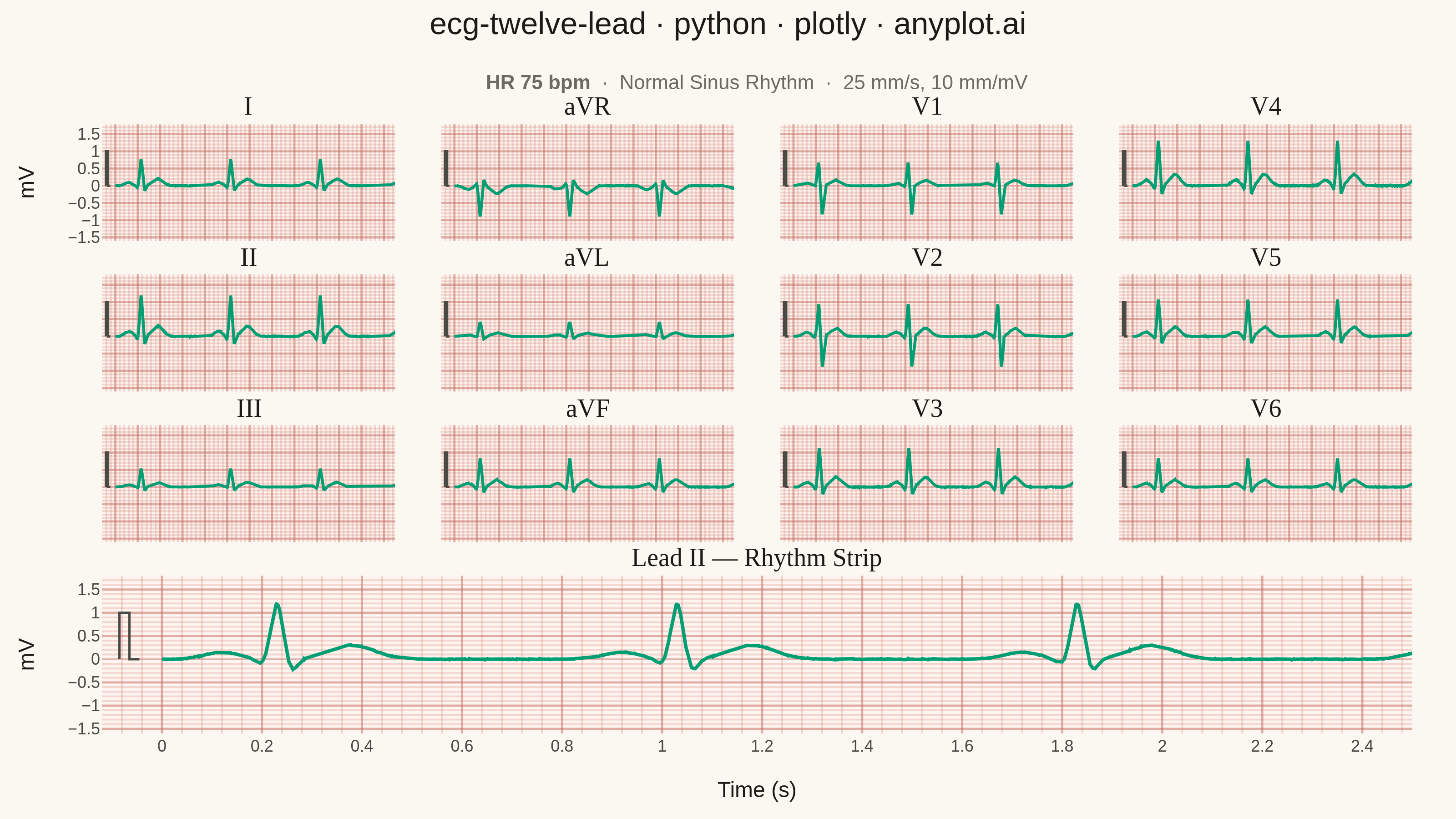
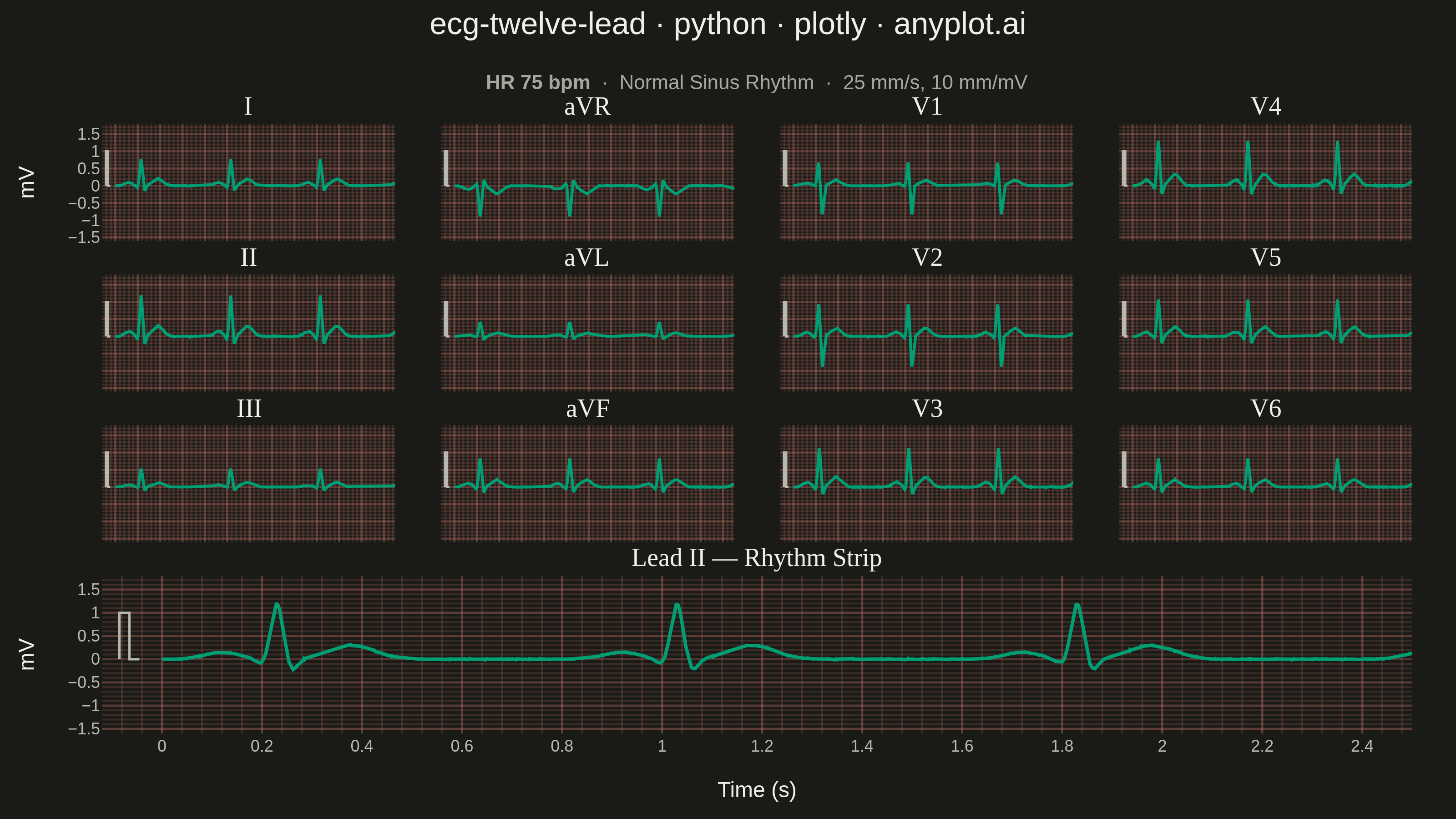
A multi-channel electrocardiogram display showing the 12 standard ECG leads arranged in clinical format. Each lead displays realistic P-QRS-T wave complexes on a medical-standard grid background with calibration markers. This visualization replicates the familiar layout used in hospitals and clinics worldwide, making it immediately recognizable to healthcare professionals and useful for medical education.
""" anyplot.ai
ecg-twelve-lead: ECG/EKG 12-Lead Waveform Display
Library: plotly 6.8.0 | Python 3.13.13
Quality: 93/100 | Updated: 2026-06-17
"""

import os

import numpy as np
import plotly.graph_objects as go
from plotly.subplots import make_subplots


# Theme-adaptive chrome (Imprint palette)
THEME = os.getenv("ANYPLOT_THEME", "light")
LIGHT = THEME == "light"

PAGE_BG = "#FAF8F1" if LIGHT else "#1A1A17"
ELEVATED_BG = "#FFFDF6" if LIGHT else "#242420"
INK = "#1A1A17" if LIGHT else "#F0EFE8"
INK_SOFT = "#4A4A44" if LIGHT else "#B8B7B0"
INK_MUTED = "#6B6A63" if LIGHT else "#A8A79F"

# ECG paper styling — printed paper on light, bedside monitor on dark.
# Both keep the medical-standard red/salmon grid the spec requires.
if LIGHT:
    PAPER_FILL = "#FFF5F0"  # warm pinkish ECG recording paper
    GRID_MINOR = "rgba(214, 150, 138, 0.32)"  # 1 mm light lines
    GRID_MAJOR = "rgba(196, 108, 96, 0.52)"  # 5 mm bold lines
    ZERO_LINE = "rgba(190, 100, 90, 0.45)"
else:
    PAPER_FILL = "#1A1A17"  # dark cardiac-monitor surface
    GRID_MINOR = "rgba(204, 120, 110, 0.18)"
    GRID_MAJOR = "rgba(214, 122, 110, 0.34)"
    ZERO_LINE = "rgba(214, 122, 110, 0.32)"

# Imprint palette position 1 — the brand green doubles as the classic
# green cardiac-monitor trace, so the single data series stays on-brand.
TRACE = "#009E73"

# Data — synthetic ECG via a simplified Gaussian P-QRS-T model
np.random.seed(42)

sampling_rate = 1000
duration = 2.5
t = np.linspace(0, duration, int(sampling_rate * duration))

# Base Lead II signal built inline (KISS — no helper functions)
beat_interval = 0.8
lead_II_signal = np.zeros_like(t)
for beat_start in np.arange(0, duration, beat_interval):
    t_shifted = t - beat_start
    mask = (t_shifted >= 0) & (t_shifted < beat_interval)
    tb = t_shifted[mask]
    lead_II_signal[mask] += (
        0.15 * np.exp(-((tb - 0.12) ** 2) / (2 * 0.035**2))  # P wave
        + (-0.12) * np.exp(-((tb - 0.20) ** 2) / (2 * 0.012**2))  # Q wave
        + 1.2 * np.exp(-((tb - 0.23) ** 2) / (2 * 0.012**2))  # R wave
        + (-0.25) * np.exp(-((tb - 0.26) ** 2) / (2 * 0.012**2))  # S wave
        + 0.3 * np.exp(-((tb - 0.38) ** 2) / (2 * 0.045**2))  # T wave
    )

lead_II_signal += np.random.normal(0, 0.005, len(t))

# Per-lead transforms deriving all 12 leads from Lead II.
# r_ratio < 0 → precordial leads with deeper S-waves (V1-V2 deepest).
lead_transforms = {
    "I": {"scale": 0.65, "t_inv": False},
    "II": {"scale": 1.0, "t_inv": False},
    "III": {"scale": 0.45, "t_inv": False},
    "aVR": {"scale": 0.75, "t_inv": True},
    "aVL": {"scale": 0.35, "t_inv": False},
    "aVF": {"scale": 0.70, "t_inv": False},
    "V1": {"scale": 0.55, "r_ratio": -1.0},
    "V2": {"scale": 0.80, "r_ratio": -0.7},
    "V3": {"scale": 0.95, "r_ratio": 0.3},
    "V4": {"scale": 1.10, "r_ratio": 0.7},
    "V5": {"scale": 0.90, "r_ratio": 0.9},
    "V6": {"scale": 0.70, "r_ratio": 1.0},
}

leads = {}
for name, params in lead_transforms.items():
    signal = lead_II_signal * params["scale"]
    if params.get("t_inv"):
        signal = -signal
    if "r_ratio" in params:
        r_ratio = params["r_ratio"]
        for beat_start in np.arange(0, duration, beat_interval):
            t_shifted = t - beat_start
            mask = (t_shifted >= 0.19) & (t_shifted < 0.28)
            if r_ratio < 0:
                # Small r, dominant deep S (rS morphology of V1-V2)
                r_component = 0.6 * np.exp(-((t_shifted - 0.22) ** 2) / (2 * 0.012**2)) * params["scale"]
                s_extra = -1.5 * np.exp(-((t_shifted - 0.25) ** 2) / (2 * 0.016**2)) * params["scale"]
                signal[mask] += r_component[mask] * abs(r_ratio)
                signal[mask] += s_extra[mask] * abs(r_ratio)
    leads[name] = signal

# Standard clinical 3x4 column order + Lead II rhythm strip
grid_layout = [["I", "aVR", "V1", "V4"], ["II", "aVL", "V2", "V5"], ["III", "aVF", "V3", "V6"]]

# Plot
fig = make_subplots(
    rows=4,
    cols=4,
    specs=[[{}, {}, {}, {}], [{}, {}, {}, {}], [{}, {}, {}, {}], [{"colspan": 4}, None, None, None]],
    row_heights=[0.23, 0.23, 0.23, 0.31],
    vertical_spacing=0.055,
    horizontal_spacing=0.035,
    subplot_titles=[
        "I",
        "aVR",
        "V1",
        "V4",
        "II",
        "aVL",
        "V2",
        "V5",
        "III",
        "aVF",
        "V3",
        "V6",
        "Lead II — Rhythm Strip",
    ],
)

# ECG signal traces with interactive hover detail
for row_idx, row_leads in enumerate(grid_layout):
    for col_idx, lead_name in enumerate(row_leads):
        fig.add_trace(
            go.Scatter(
                x=t,
                y=leads[lead_name],
                mode="lines",
                line={"color": TRACE, "width": 1.6},
                showlegend=False,
                name=lead_name,
                hovertemplate=f"<b>{lead_name}</b><br>Time: %{{x:.3f}} s<br>Voltage: %{{y:.2f}} mV<extra></extra>",
            ),
            row=row_idx + 1,
            col=col_idx + 1,
        )

# Full-length Lead II rhythm strip
fig.add_trace(
    go.Scatter(
        x=t,
        y=leads["II"],
        mode="lines",
        line={"color": TRACE, "width": 1.9},
        showlegend=False,
        name="Lead II",
        hovertemplate="<b>Lead II</b><br>Time: %{x:.3f} s<br>Voltage: %{y:.2f} mV<extra></extra>",
    ),
    row=4,
    col=1,
)

# 1 mV / 0.2 s calibration pulse at the left margin of every panel
cal_t = np.array([0.0, 0.0, 0.02, 0.02, 0.04, 0.04]) - 0.085
cal_v = np.array([0.0, 1.0, 1.0, 0.0, 0.0, 0.0])

for row_idx in range(4):
    cols = [1, 2, 3, 4] if row_idx < 3 else [1]
    for col_idx in cols:
        fig.add_trace(
            go.Scatter(
                x=cal_t,
                y=cal_v,
                mode="lines",
                line={"color": INK_SOFT, "width": 1.3},
                showlegend=False,
                hoverinfo="skip",
            ),
            row=row_idx + 1,
            col=col_idx,
        )

# Style — medical ECG grid on every axis
for row_idx in range(1, 5):
    cols = [1, 2, 3, 4] if row_idx <= 3 else [1]
    for col_idx in cols:
        fig.update_xaxes(
            range=[-0.12, duration],
            dtick=0.2,
            minor={"dtick": 0.04, "gridcolor": GRID_MINOR, "gridwidth": 1, "showgrid": True},
            gridcolor=GRID_MAJOR,
            gridwidth=1.2,
            showgrid=True,
            zeroline=False,
            showticklabels=(row_idx == 4),
            tickfont={"size": 9, "color": INK_SOFT},
            ticks="",
            row=row_idx,
            col=col_idx,
        )
        fig.update_yaxes(
            range=[-1.6, 1.8],
            dtick=0.5,
            minor={"dtick": 0.1, "gridcolor": GRID_MINOR, "gridwidth": 1, "showgrid": True},
            gridcolor=GRID_MAJOR,
            gridwidth=1.2,
            showgrid=True,
            zeroline=True,
            zerolinecolor=ZERO_LINE,
            zerolinewidth=1,
            showticklabels=False,
            ticks="",
            row=row_idx,
            col=col_idx,
        )

# Voltage / time axis labels on the reference panels
fig.update_yaxes(
    showticklabels=True,
    tickfont={"size": 9, "color": INK_SOFT},
    title_text="mV",
    title_font={"size": 12, "color": INK},
    row=1,
    col=1,
)
fig.update_yaxes(
    showticklabels=True,
    tickfont={"size": 9, "color": INK_SOFT},
    title_text="mV",
    title_font={"size": 12, "color": INK},
    row=4,
    col=1,
)
fig.update_xaxes(
    title_text="Time (s)", title_font={"size": 12, "color": INK}, tickfont={"size": 9, "color": INK_SOFT}, row=4, col=1
)

fig.update_layout(
    title={
        "text": "ecg-twelve-lead · python · plotly · anyplot.ai",
        "font": {"size": 17, "color": INK},
        "x": 0.5,
        "xanchor": "center",
        "y": 0.985,
    },
    paper_bgcolor=PAGE_BG,
    plot_bgcolor=PAPER_FILL,
    font={"color": INK},
    showlegend=False,
    margin={"l": 56, "r": 24, "t": 68, "b": 40},
    hoverlabel={"bgcolor": ELEVATED_BG, "font_size": 13, "font_color": INK, "bordercolor": INK_SOFT},
    hovermode="closest",
)

# Lead-name subplot titles — bold and legible for clinical identification
fig.update_annotations(font={"size": 14, "color": INK, "family": "Arial Black"})

# Clinical context strip below the title
fig.add_annotation(
    text="<b>HR 75 bpm</b>  ·  Normal Sinus Rhythm  ·  25 mm/s, 10 mm/mV",
    xref="paper",
    yref="paper",
    x=0.5,
    y=1.045,
    showarrow=False,
    font={"size": 11, "color": INK_MUTED, "family": "Arial"},
    xanchor="center",
    yanchor="bottom",
)

# Save
fig.write_image(f"plot-{THEME}.png", width=800, height=450, scale=4)
fig.write_html(f"plot-{THEME}.html", include_plotlyjs="cdn")
Runnable source as JSON, for any HTTP client: https://api.anyplot.ai/specs/ecg-twelve-lead/plotly/code. Any spec id and library id listed in llms-full.txt fit the same URL shape; every URL below is complete and callable.
{
  "spec_id": "ecg-twelve-lead",
  "language": "python",
  "library": "plotly",
  "page": "https://anyplot.ai/ecg-twelve-lead/python/plotly",
  "hub": "https://anyplot.ai/ecg-twelve-lead",
  "code_json": "https://api.anyplot.ai/specs/ecg-twelve-lead/plotly/code",
  "spec_json": "https://api.anyplot.ai/specs/ecg-twelve-lead",
  "render_light_png": "https://storage.googleapis.com/anyplot-images/plots/ecg-twelve-lead/python/plotly/plot-light.png",
  "render_dark_png": "https://storage.googleapis.com/anyplot-images/plots/ecg-twelve-lead/python/plotly/plot-dark.png",
  "interactive_light_html": "https://storage.googleapis.com/anyplot-images/plots/ecg-twelve-lead/python/plotly/plot-light.html",
  "interactive_dark_html": "https://storage.googleapis.com/anyplot-images/plots/ecg-twelve-lead/python/plotly/plot-dark.html",
  "quality_score": 93.0,
  "license": "MIT",
  "guide": "https://anyplot.ai/llms.txt"
}
Part of ECG/EKG 12-Lead Waveform Display on anyplot.ai.