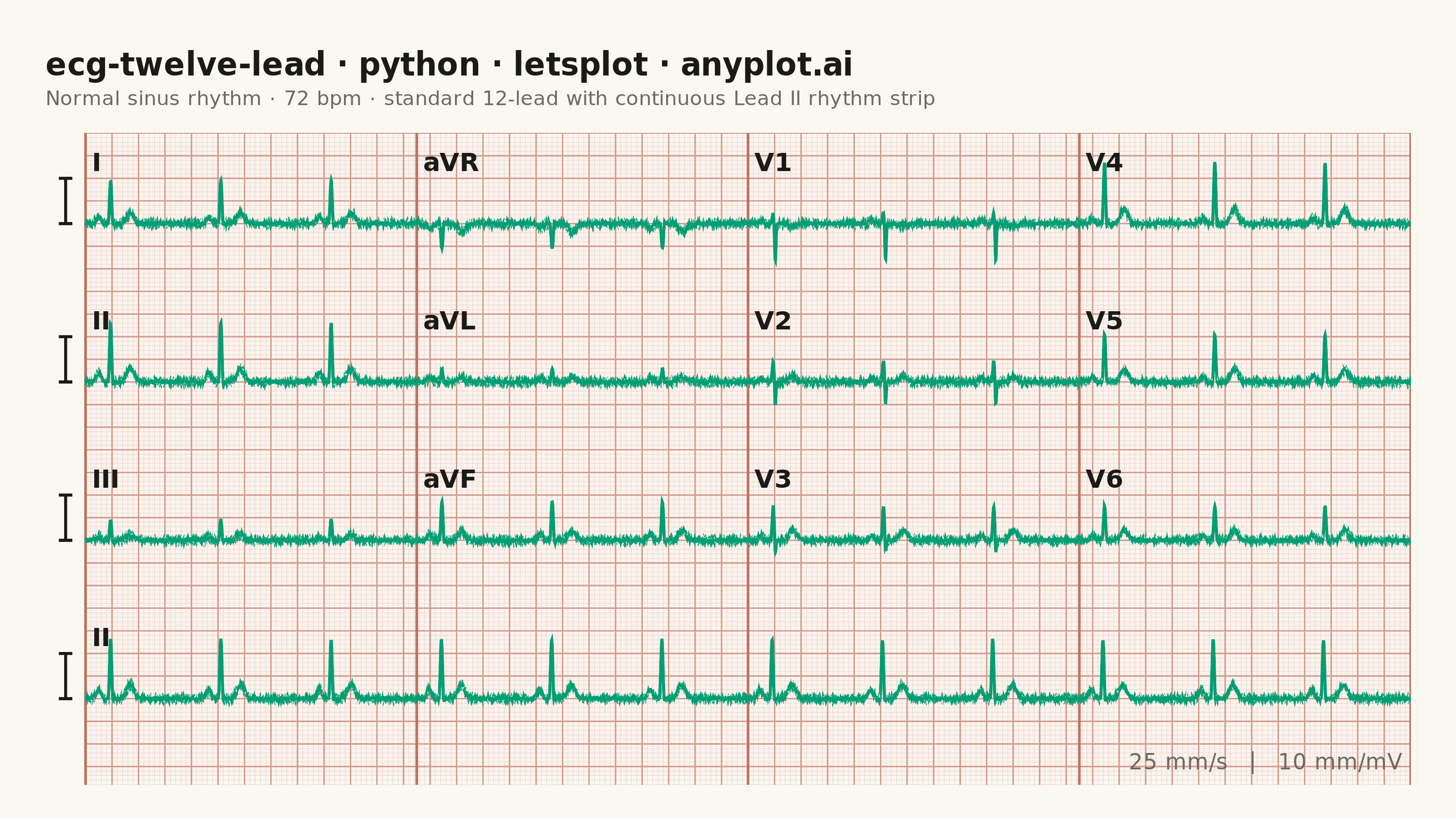
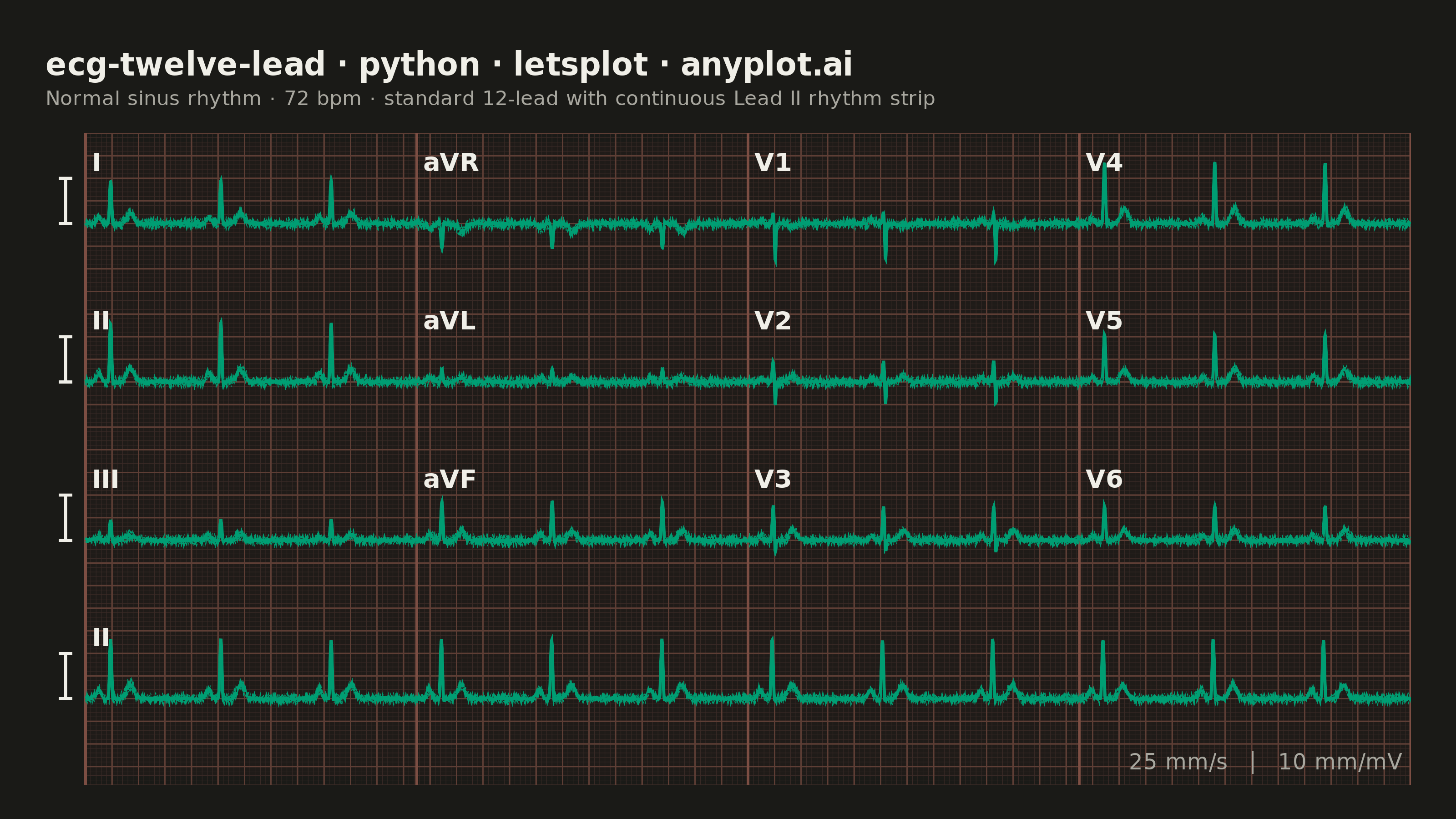
A multi-channel electrocardiogram display showing the 12 standard ECG leads arranged in clinical format. Each lead displays realistic P-QRS-T wave complexes on a medical-standard grid background with calibration markers. This visualization replicates the familiar layout used in hospitals and clinics worldwide, making it immediately recognizable to healthcare professionals and useful for medical education.
""" anyplot.ai
ecg-twelve-lead: ECG/EKG 12-Lead Waveform Display
Library: letsplot 4.10.1 | Python 3.13.13
Quality: 93/100 | Updated: 2026-06-17
"""

import os

import numpy as np
import pandas as pd
from lets_plot import (
    LetsPlot,
    aes,
    element_blank,
    element_rect,
    element_text,
    geom_line,
    geom_rect,
    geom_segment,
    geom_text,
    ggplot,
    ggsize,
    labs,
    layer_tooltips,
    scale_x_continuous,
    scale_y_continuous,
    theme,
)
from lets_plot.export import ggsave


LetsPlot.setup_html()

# Theme-adaptive chrome (Imprint palette + theme tokens)
THEME = os.getenv("ANYPLOT_THEME", "light")
PAGE_BG = "#FAF8F1" if THEME == "light" else "#1A1A17"
INK = "#1A1A17" if THEME == "light" else "#F0EFE8"
INK_MUTED = "#6B6A63" if THEME == "light" else "#A8A79F"

# ECG-paper grid — classic red ruling, kept as theme-adaptive chrome so the
# iconic medical look survives on both the warm-cream and warm-black surfaces.
PAPER_TINT = "#FBF0EB" if THEME == "light" else "#241C19"
GRID_MINOR = "#EBD2CB" if THEME == "light" else "#3A2A26"
GRID_MAJOR = "#D49B8E" if THEME == "light" else "#5E3E35"
GRID_COL = "#BC7563" if THEME == "light" else "#7C4E43"

# ECG trace = Imprint brand green (position 1) — identical in both themes, only
# chrome flips. Green tracings are a real patient-monitor convention.
TRACE = "#009E73"

# Data - Synthetic ECG (Normal Sinus Rhythm)
np.random.seed(42)

fs = 500
strip_duration = 2.5
n_strip = int(fs * strip_duration)
t_strip = np.linspace(0, strip_duration, n_strip, endpoint=False)

hr = 72
beat_period = 60.0 / hr
n_beat = int(fs * beat_period)
t_beat = np.linspace(0, beat_period, n_beat, endpoint=False)

# ECG waveform components (Gaussian model for P-QRS-T complex)
p_comp = np.exp(-((t_beat - 0.10) ** 2) / (2 * 0.018**2))
q_comp = np.exp(-((t_beat - 0.175) ** 2) / (2 * 0.004**2))
r_comp = np.exp(-((t_beat - 0.19) ** 2) / (2 * 0.008**2))
s_comp = np.exp(-((t_beat - 0.205) ** 2) / (2 * 0.005**2))
tw_comp = np.exp(-((t_beat - 0.34) ** 2) / (2 * 0.028**2))

# Per-lead amplitudes [P, Q, R, S, T] in mV
lead_weights = {
    "I": [0.15, -0.07, 0.95, -0.10, 0.22],
    "II": [0.20, -0.10, 1.30, -0.15, 0.30],
    "III": [0.07, -0.05, 0.45, -0.08, 0.12],
    "aVR": [-0.12, 0.06, -0.55, 0.10, -0.18],
    "aVL": [0.09, -0.03, 0.28, -0.05, 0.10],
    "aVF": [0.14, -0.07, 0.85, -0.12, 0.20],
    "V1": [0.07, 0.00, 0.22, -0.85, -0.06],
    "V2": [0.09, -0.02, 0.45, -0.55, 0.12],
    "V3": [0.10, -0.06, 0.75, -0.35, 0.22],
    "V4": [0.12, -0.10, 1.35, -0.18, 0.32],
    "V5": [0.12, -0.08, 1.05, -0.08, 0.28],
    "V6": [0.10, -0.05, 0.75, -0.04, 0.22],
}

# Clinical 3x4 grid layout: (row, col)
grid_positions = {
    "I": (0, 0),
    "aVR": (0, 1),
    "V1": (0, 2),
    "V4": (0, 3),
    "II": (1, 0),
    "aVL": (1, 1),
    "V2": (1, 2),
    "V5": (1, 3),
    "III": (2, 0),
    "aVF": (2, 1),
    "V3": (2, 2),
    "V6": (2, 3),
}

row_spacing = 3.5
n_rows = 3
total_time = 4 * strip_duration

# Generate ECG traces with grid offsets
all_traces = []
label_records = []

for lead_name, w in lead_weights.items():
    one_beat = w[0] * p_comp + w[1] * q_comp + w[2] * r_comp + w[3] * s_comp + w[4] * tw_comp
    signal = np.tile(one_beat, int(np.ceil(n_strip / n_beat)) + 1)[:n_strip]
    signal += np.random.normal(0, 0.015, n_strip)

    row, col = grid_positions[lead_name]
    x_vals = t_strip + col * strip_duration
    y_baseline = (n_rows - 1 - row) * row_spacing + row_spacing

    all_traces.append(pd.DataFrame({"time": x_vals, "voltage": signal + y_baseline, "lead": lead_name}))
    label_records.append({"time": x_vals[0] + 0.05, "voltage": y_baseline + 1.35, "label": lead_name})

# Lead II rhythm strip across the bottom (full 10 seconds)
n_full = int(fs * total_time)
t_full = np.linspace(0, total_time, n_full, endpoint=False)
w_ii = lead_weights["II"]
one_beat_ii = w_ii[0] * p_comp + w_ii[1] * q_comp + w_ii[2] * r_comp + w_ii[3] * s_comp + w_ii[4] * tw_comp
signal_ii = np.tile(one_beat_ii, int(np.ceil(n_full / n_beat)) + 1)[:n_full]
signal_ii += np.random.normal(0, 0.015, n_full)

rhythm_baseline = 0.0
all_traces.append(pd.DataFrame({"time": t_full, "voltage": signal_ii + rhythm_baseline, "lead": "II_rhythm"}))
label_records.append({"time": 0.05, "voltage": rhythm_baseline + 1.35, "label": "II"})

df = pd.concat(all_traces, ignore_index=True)
labels_df = pd.DataFrame(label_records)

# 1mV calibration pulses at left margin of each row + rhythm strip
cal_records = []
for row_idx in range(n_rows):
    y_base = (n_rows - 1 - row_idx) * row_spacing + row_spacing
    cal_x = -0.15
    cal_records.extend(
        [
            {"x": cal_x, "y": y_base, "xend": cal_x, "yend": y_base + 1.0},
            {"x": cal_x - 0.05, "y": y_base, "xend": cal_x + 0.05, "yend": y_base},
            {"x": cal_x - 0.05, "y": y_base + 1.0, "xend": cal_x + 0.05, "yend": y_base + 1.0},
        ]
    )
# Rhythm strip calibration
cal_records.extend(
    [
        {"x": -0.15, "y": rhythm_baseline, "xend": -0.15, "yend": rhythm_baseline + 1.0},
        {"x": -0.20, "y": rhythm_baseline, "xend": -0.10, "yend": rhythm_baseline},
        {"x": -0.20, "y": rhythm_baseline + 1.0, "xend": -0.10, "yend": rhythm_baseline + 1.0},
    ]
)
cal_df = pd.DataFrame(cal_records)

# Scale annotation text (bumped size — prev review flagged it as slightly small)
scale_df = pd.DataFrame({"x": [total_time - 0.05], "y": [rhythm_baseline - 1.4], "label": ["25 mm/s   |   10 mm/mV"]})

# ECG paper grid extents
y_min = rhythm_baseline - 1.9
y_max = (n_rows - 1) * row_spacing + row_spacing + 2.0

# Paper-region backgrounds using geom_rect (lets-plot distinctive feature)
row_rects = []
for row_idx in range(n_rows):
    y_base = (n_rows - 1 - row_idx) * row_spacing + row_spacing
    row_rects.append(
        {"xmin": 0, "xmax": total_time, "ymin": y_base - 1.7, "ymax": y_base + 1.8, "region": f"Row {row_idx + 1}"}
    )
row_rects.append(
    {
        "xmin": 0,
        "xmax": total_time,
        "ymin": rhythm_baseline - 1.7,
        "ymax": rhythm_baseline + 1.8,
        "region": "Rhythm Strip",
    }
)
row_rects_df = pd.DataFrame(row_rects)

# Minor grid (1mm equivalent: 0.04s horizontal, 0.1mV vertical)
minor_x_vals = np.arange(0, total_time + 0.01, 0.04)
minor_y_vals = np.arange(np.floor(y_min), y_max + 0.01, 0.1)
minor_v = pd.DataFrame({"x": minor_x_vals, "xend": minor_x_vals, "y": y_min, "yend": y_max})
minor_h = pd.DataFrame({"y": minor_y_vals, "yend": minor_y_vals, "x": 0.0, "xend": total_time})

# Major grid (5mm equivalent: 0.2s horizontal, 0.5mV vertical)
major_x_vals = np.arange(0, total_time + 0.01, 0.2)
major_y_vals = np.arange(np.floor(y_min), y_max + 0.01, 0.5)
major_v = pd.DataFrame({"x": major_x_vals, "xend": major_x_vals, "y": y_min, "yend": y_max})
major_h = pd.DataFrame({"y": major_y_vals, "yend": major_y_vals, "x": 0.0, "xend": total_time})

# Column separator lines (thicker at 2.5s boundaries)
col_boundaries = [strip_duration * i for i in range(5)]
col_sep = pd.DataFrame({"x": col_boundaries, "xend": col_boundaries, "y": y_min, "yend": y_max})

# Plot
plot = (
    ggplot()
    # Paper-region backgrounds (lets-plot geom_rect)
    + geom_rect(
        aes(xmin="xmin", xmax="xmax", ymin="ymin", ymax="ymax"),
        data=row_rects_df,
        fill=PAPER_TINT,
        alpha=0.5,
        color="rgba(0,0,0,0)",
        tooltips=layer_tooltips().line("@region"),
        inherit_aes=False,
    )
    # Minor grid
    + geom_segment(
        aes(x="x", y="y", xend="xend", yend="yend"), data=minor_v, color=GRID_MINOR, size=0.1, inherit_aes=False
    )
    + geom_segment(
        aes(x="x", y="y", xend="xend", yend="yend"), data=minor_h, color=GRID_MINOR, size=0.1, inherit_aes=False
    )
    # Major grid
    + geom_segment(
        aes(x="x", y="y", xend="xend", yend="yend"), data=major_v, color=GRID_MAJOR, size=0.3, inherit_aes=False
    )
    + geom_segment(
        aes(x="x", y="y", xend="xend", yend="yend"), data=major_h, color=GRID_MAJOR, size=0.3, inherit_aes=False
    )
    # Column separators
    + geom_segment(
        aes(x="x", y="y", xend="xend", yend="yend"), data=col_sep, color=GRID_COL, size=0.6, inherit_aes=False
    )
    # 1mV calibration pulses
    + geom_segment(aes(x="x", y="y", xend="xend", yend="yend"), data=cal_df, color=INK, size=0.7, inherit_aes=False)
    # ECG traces with interactive tooltips (lets-plot layer_tooltips)
    + geom_line(
        aes(x="time", y="voltage", group="lead"),
        data=df,
        color=TRACE,
        size=0.7,
        tooltips=layer_tooltips().line("Lead: @lead").format("time", ".2f").line("Time: @time s"),
    )
    # Lead labels
    + geom_text(
        aes(x="time", y="voltage", label="label"),
        data=labels_df,
        color=INK,
        size=7,
        fontface="bold",
        hjust=0,
        inherit_aes=False,
    )
    # Scale annotation
    + geom_text(aes(x="x", y="y", label="label"), data=scale_df, color=INK_MUTED, size=6, hjust=1, inherit_aes=False)
    # Scales
    + scale_x_continuous(limits=[-0.3, total_time], expand=[0, 0])
    + scale_y_continuous(limits=[y_min, y_max], expand=[0, 0])
    + labs(
        title="ecg-twelve-lead · python · letsplot · anyplot.ai",
        subtitle="Normal sinus rhythm · 72 bpm · standard 12-lead with continuous Lead II rhythm strip",
    )
    # Theme - ECG paper style
    + theme(
        plot_title=element_text(size=17, face="bold", color=INK, margin=[0, 0, 4, 0]),
        plot_subtitle=element_text(size=11, color=INK_MUTED, margin=[0, 0, 10, 0]),
        axis_title=element_blank(),
        axis_text=element_blank(),
        axis_ticks=element_blank(),
        axis_line=element_blank(),
        panel_background=element_rect(fill=PAGE_BG, color="rgba(0,0,0,0)"),
        plot_background=element_rect(fill=PAGE_BG, color=PAGE_BG),
        panel_grid=element_blank(),
        plot_margin=[28, 22, 16, 22],
        legend_position="none",
    )
    + ggsize(800, 450)
)

# Save (scale 4x -> 3200 x 1800 px)
ggsave(plot, f"plot-{THEME}.png", path=".", scale=4)
ggsave(plot, f"plot-{THEME}.html", path=".")
Runnable source as JSON, for any HTTP client: https://api.anyplot.ai/specs/ecg-twelve-lead/letsplot/code. Any spec id and library id listed in llms-full.txt fit the same URL shape; every URL below is complete and callable.
{
  "spec_id": "ecg-twelve-lead",
  "language": "python",
  "library": "letsplot",
  "page": "https://anyplot.ai/ecg-twelve-lead/python/letsplot",
  "hub": "https://anyplot.ai/ecg-twelve-lead",
  "code_json": "https://api.anyplot.ai/specs/ecg-twelve-lead/letsplot/code",
  "spec_json": "https://api.anyplot.ai/specs/ecg-twelve-lead",
  "render_light_png": "https://storage.googleapis.com/anyplot-images/plots/ecg-twelve-lead/python/letsplot/plot-light.png",
  "render_dark_png": "https://storage.googleapis.com/anyplot-images/plots/ecg-twelve-lead/python/letsplot/plot-dark.png",
  "interactive_light_html": "https://storage.googleapis.com/anyplot-images/plots/ecg-twelve-lead/python/letsplot/plot-light.html",
  "interactive_dark_html": "https://storage.googleapis.com/anyplot-images/plots/ecg-twelve-lead/python/letsplot/plot-dark.html",
  "quality_score": 93.0,
  "license": "MIT",
  "guide": "https://anyplot.ai/llms.txt"
}
Part of ECG/EKG 12-Lead Waveform Display on anyplot.ai.