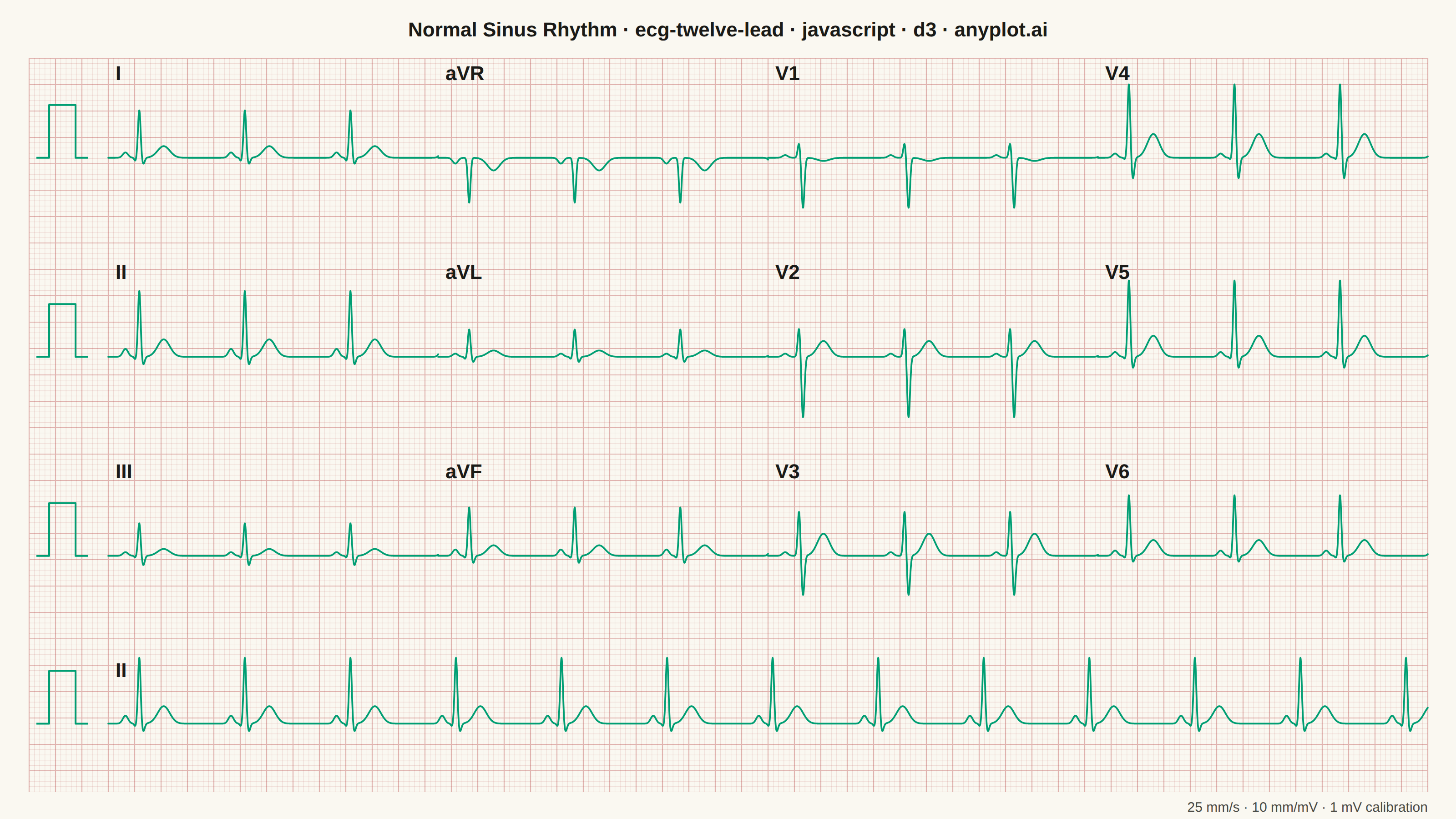
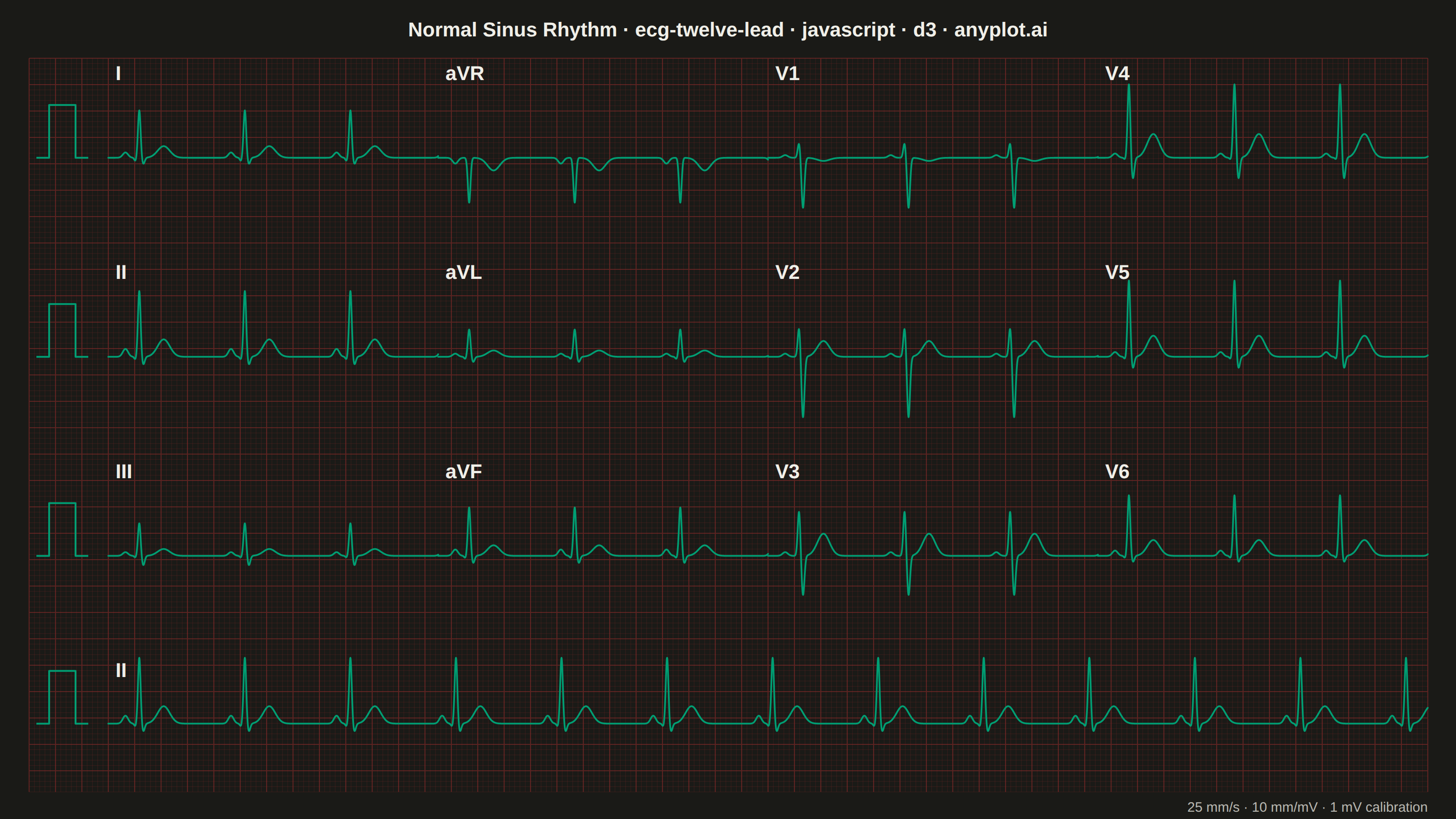
A multi-channel electrocardiogram display showing the 12 standard ECG leads arranged in clinical format. Each lead displays realistic P-QRS-T wave complexes on a medical-standard grid background with calibration markers. This visualization replicates the familiar layout used in hospitals and clinics worldwide, making it immediately recognizable to healthcare professionals and useful for medical education.
// anyplot.ai
// ecg-twelve-lead: ECG/EKG 12-Lead Waveform Display
// Library: d3 7.9.0 | JavaScript 22.22.3
// Quality: 91/100 | Created: 2026-06-17
//# anyplot-orientation: landscape
// anyplot.ai
// ecg-twelve-lead: ECG/EKG 12-Lead Waveform Display
// Library: d3 7.9.0 | JavaScript 22
// Quality: pending | Created: 2026-06-17

const t = window.ANYPLOT_TOKENS;
const { width, height } = window.ANYPLOT_SIZE;

// --- ECG paper geometry ------------------------------------------------------
// Standard clinical scale: 25 mm/s horizontal, 10 mm/mV vertical. One small grid
// square = 1 mm, one bold square = 5 mm. pxPerMm fixes the physical scale; every
// downstream measurement (strip width, voltage, calibration pulse) derives from it.
const pxPerMm = 5.8;
const pxPerMv = 10 * pxPerMm; // 10 mm/mV
const mmPerSec = 25; // paper speed
const pxPerSec = mmPerSec * pxPerMm; // 145 px/s
const stripSec = 2.5; // seconds shown per lead cell (2.5 s × 4 cols = 10 s)
const calGutterMm = 15; // left margin reserved for the 1 mV calibration pulse

// Continuous pink grid spans the whole plot rectangle, like real ECG paper.
const gridTop = 64;
const gridWmm = calGutterMm + 4 * stripSec * mmPerSec; // 15 + 250 = 265 mm
const gridWpx = gridWmm * pxPerMm;
const gridLeft = Math.round((width - gridWpx) / 2);
const gridHmm = Math.floor((height - gridTop - 26) / pxPerMm);
const gridHpx = gridHmm * pxPerMm;
const gridRight = gridLeft + gridWpx;
const gridBottom = gridTop + gridHpx;

// Vertical split: three rows of leads + one full-width Lead II rhythm strip.
const rhythmH = 150;
const leadH = (gridHpx - rhythmH) / 3;
const colWpx = stripSec * pxPerSec; // 362.5 px per 2.5 s cell
const colX0 = (c) => gridLeft + calGutterMm * pxPerMm + c * colWpx;
const rowBaseline = (r) => gridTop + leadH * (r + 0.5);
const rhythmBaseline = gridTop + 3 * leadH + rhythmH / 2;

// Standard clinical 3×4 placement (columns I/aVR/V1/V4 · II/aVL/V2/V5 · III/aVF/V3/V6).
const layout = [
  ["I", "aVR", "V1", "V4"],
  ["II", "aVL", "V2", "V5"],
  ["III", "aVF", "V3", "V6"],
];

// --- Synthetic normal sinus rhythm ------------------------------------------
// Each beat is a sum of Gaussian P-Q-R-S-T deflections (a compact analogue of the
// McSharry ECG model). Per-lead coefficients (mV) set the signed amplitude of each
// wave, reproducing the textbook morphology: inverted aVR, rS in V1 progressing to
// a tall R in V5/V6, and the limb-lead pattern. Amplitudes sit in normal ranges
// (P ~0.1–0.25 mV, QRS ~0.5–1.5 mV, T ~0.1–0.5 mV).
const beatSec = 0.8; // ~75 bpm
const waves = [
  { key: "P", mu: 0.13, sig: 0.02 },
  { key: "Q", mu: 0.205, sig: 0.008 },
  { key: "R", mu: 0.235, sig: 0.01 },
  { key: "S", mu: 0.265, sig: 0.011 },
  { key: "T", mu: 0.42, sig: 0.046 },
];
const coef = {
  I: { P: 0.1, Q: -0.06, R: 0.9, S: -0.12, T: 0.22 },
  II: { P: 0.15, Q: -0.05, R: 1.25, S: -0.15, T: 0.33 },
  III: { P: 0.07, Q: -0.03, R: 0.62, S: -0.18, T: 0.13 },
  aVR: { P: -0.11, Q: 0, R: -0.85, S: 0, T: -0.24 },
  aVL: { P: 0.06, Q: -0.04, R: 0.52, S: -0.1, T: 0.12 },
  aVF: { P: 0.12, Q: -0.04, R: 0.92, S: -0.14, T: 0.2 },
  V1: { P: 0.05, Q: 0, R: 0.28, S: -0.95, T: -0.06 },
  V2: { P: 0.06, Q: 0, R: 0.55, S: -1.15, T: 0.3 },
  V3: { P: 0.07, Q: 0, R: 0.85, S: -0.75, T: 0.42 },
  V4: { P: 0.08, Q: -0.03, R: 1.4, S: -0.4, T: 0.45 },
  V5: { P: 0.09, Q: -0.04, R: 1.45, S: -0.22, T: 0.4 },
  V6: { P: 0.1, Q: -0.04, R: 1.15, S: -0.12, T: 0.3 },
};

const ecg = (time, lead) => {
  const tau = ((time % beatSec) + beatSec) % beatSec;
  let v = 0;
  for (const w of waves) {
    const a = coef[lead][w.key];
    if (a) v += a * Math.exp(-((tau - w.mu) ** 2) / (2 * w.sig * w.sig));
  }
  return v;
};

// 1000 Hz sampling (2500 samples / 2.5 s strip), matching the spec acquisition rate.
const dt = 0.001;
const sample = (lead, dur) => {
  const pts = [];
  for (let time = 0; time <= dur + 1e-9; time += dt) pts.push({ t: time, v: ecg(time, lead) });
  return pts;
};

// d3.scaleLinear carries the physical ECG calibration in measured units: seconds→px
// at 25 mm/s and mV→px at 10 mm/mV. Each cell reuses the same scales, offset by its
// own (x0, yb) origin, so the d3.line accessors read in clinical units, not pixels.
const xScale = d3.scaleLinear().domain([0, 1]).range([0, pxPerSec]);
const vScale = d3.scaleLinear().domain([0, 1]).range([0, pxPerMv]);
const traceLine = (x0, yb) =>
  d3
    .line()
    .x((d) => x0 + xScale(d.t))
    .y((d) => yb - vScale(d.v));

// --- SVG mount ---------------------------------------------------------------
const svg = d3
  .select("#container")
  .append("svg")
  .attr("width", width)
  .attr("height", height);

// --- ECG paper grid (Imprint matte-red #AE3030, the palette's red anchor) -----
const major = (l) => l % 5 === 0;
let minorD = "";
let majorD = "";
const nCols = Math.floor(gridWpx / pxPerMm);
const nRows = Math.floor(gridHpx / pxPerMm);
for (let mm = 0; mm <= nCols; mm++) {
  const x = gridLeft + mm * pxPerMm;
  const seg = `M${x},${gridTop}V${gridBottom}`;
  if (major(mm)) majorD += seg;
  else minorD += seg;
}
for (let mm = 0; mm <= nRows; mm++) {
  const y = gridTop + mm * pxPerMm;
  const seg = `M${gridLeft},${y}H${gridRight}`;
  if (major(mm)) majorD += seg;
  else minorD += seg;
}
const minorOpacity = t.theme === "light" ? 0.16 : 0.22;
const majorOpacity = t.theme === "light" ? 0.34 : 0.46;
svg
  .append("path")
  .attr("d", minorD)
  .attr("stroke", "#AE3030")
  .attr("stroke-width", 0.5)
  .attr("stroke-opacity", minorOpacity)
  .attr("fill", "none");
svg
  .append("path")
  .attr("d", majorD)
  .attr("stroke", "#AE3030")
  .attr("stroke-width", 1.1)
  .attr("stroke-opacity", majorOpacity)
  .attr("fill", "none");

// --- Calibration pulse + waveform trace --------------------------------------
// Each row opens with a 1 mV (10 mm) step pulse in the left gutter, the standard
// reference mark. Trace and pulse share the brand-green ink (Imprint position 1).
const BRAND = t.palette[0];
const calAmp = 1.0 * pxPerMv; // 1 mV
const calPulse = (yb) => {
  const x = gridLeft + 8;
  const w = 5 * pxPerMm; // 5 mm flat top
  return `M${x},${yb}H${x + 14}V${yb - calAmp}H${x + 14 + w}V${yb}H${x + 14 + w + 14}`;
};
const drawCal = (yb) =>
  svg
    .append("path")
    .attr("d", calPulse(yb))
    .attr("stroke", BRAND)
    .attr("stroke-width", 2)
    .attr("fill", "none")
    .attr("stroke-linejoin", "round");
const drawTrace = (pts, x0, yb) =>
  svg
    .append("path")
    .attr("d", traceLine(x0, yb)(pts))
    .attr("stroke", BRAND)
    .attr("stroke-width", 1.9)
    .attr("fill", "none")
    .attr("stroke-linejoin", "round")
    .attr("stroke-linecap", "round");

// 12 lead cells
layout.forEach((row, r) => {
  const yb = rowBaseline(r);
  drawCal(yb);
  row.forEach((lead, c) => {
    drawTrace(sample(lead, stripSec), colX0(c), yb);
    svg
      .append("text")
      .attr("x", colX0(c) + 8)
      .attr("y", yb - leadH / 2 + 24)
      .attr("fill", t.ink)
      .style("font-size", "22px")
      .style("font-weight", "700")
      .text(lead);
  });
});

// Full-length Lead II rhythm strip across the bottom (10 s continuous)
drawCal(rhythmBaseline);
drawTrace(sample("II", 4 * stripSec), colX0(0), rhythmBaseline);
svg
  .append("text")
  .attr("x", colX0(0) + 8)
  .attr("y", rhythmBaseline - rhythmH / 2 + 24)
  .attr("fill", t.ink)
  .style("font-size", "22px")
  .style("font-weight", "700")
  .text("II");

// --- Title + scale footnote --------------------------------------------------
const title = "Normal Sinus Rhythm · ecg-twelve-lead · javascript · d3 · anyplot.ai";
const titleSize = title.length > 67 ? Math.max(14, Math.round((22 * 67) / title.length)) : 22;
svg
  .append("text")
  .attr("x", width / 2)
  .attr("y", 40)
  .attr("text-anchor", "middle")
  .attr("fill", t.ink)
  .style("font-size", `${titleSize}px`)
  .style("font-weight", "600")
  .text(title);

svg
  .append("text")
  .attr("x", gridRight)
  .attr("y", height - 8)
  .attr("text-anchor", "end")
  .attr("fill", t.inkSoft)
  .style("font-size", "15px")
  .text("25 mm/s · 10 mm/mV · 1 mV calibration");
Runnable source as JSON, for any HTTP client: https://api.anyplot.ai/specs/ecg-twelve-lead/d3/code. Any spec id and library id listed in llms-full.txt fit the same URL shape; every URL below is complete and callable.
{
  "spec_id": "ecg-twelve-lead",
  "language": "javascript",
  "library": "d3",
  "page": "https://anyplot.ai/ecg-twelve-lead/javascript/d3",
  "hub": "https://anyplot.ai/ecg-twelve-lead",
  "code_json": "https://api.anyplot.ai/specs/ecg-twelve-lead/d3/code",
  "spec_json": "https://api.anyplot.ai/specs/ecg-twelve-lead",
  "render_light_png": "https://storage.googleapis.com/anyplot-images/plots/ecg-twelve-lead/javascript/d3/plot-light.png",
  "render_dark_png": "https://storage.googleapis.com/anyplot-images/plots/ecg-twelve-lead/javascript/d3/plot-dark.png",
  "interactive_light_html": "https://storage.googleapis.com/anyplot-images/plots/ecg-twelve-lead/javascript/d3/plot-light.html",
  "interactive_dark_html": "https://storage.googleapis.com/anyplot-images/plots/ecg-twelve-lead/javascript/d3/plot-dark.html",
  "quality_score": 91.0,
  "license": "MIT",
  "guide": "https://anyplot.ai/llms.txt"
}
Part of ECG/EKG 12-Lead Waveform Display on anyplot.ai.