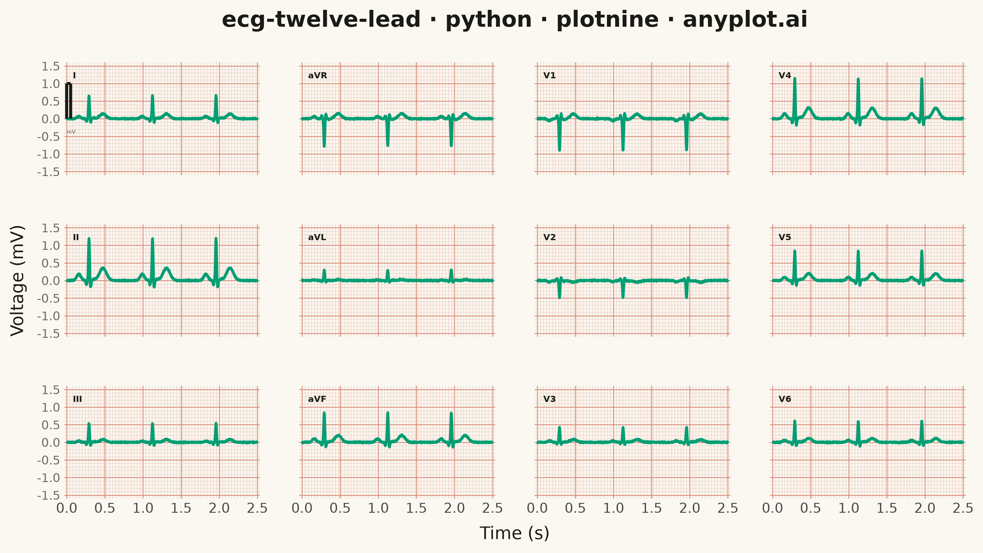
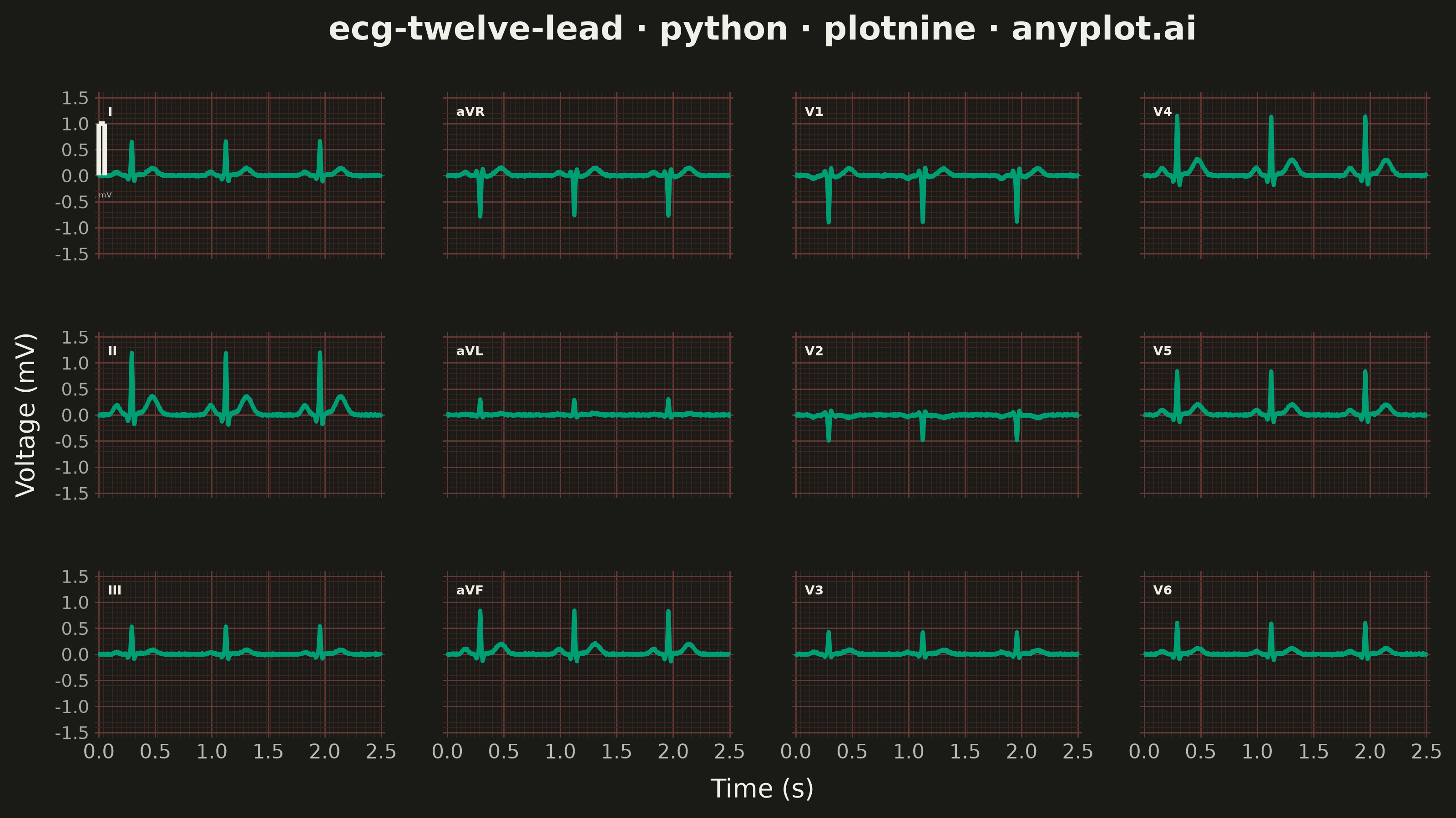
A multi-channel electrocardiogram display showing the 12 standard ECG leads arranged in clinical format. Each lead displays realistic P-QRS-T wave complexes on a medical-standard grid background with calibration markers. This visualization replicates the familiar layout used in hospitals and clinics worldwide, making it immediately recognizable to healthcare professionals and useful for medical education.
""" anyplot.ai
ecg-twelve-lead: ECG/EKG 12-Lead Waveform Display
Library: plotnine 0.15.7 | Python 3.13.13
Quality: 90/100 | Updated: 2026-06-17
"""

import os

import numpy as np
import pandas as pd
from plotnine import (
    aes,
    coord_cartesian,
    element_blank,
    element_line,
    element_rect,
    element_text,
    facet_wrap,
    geom_line,
    geom_segment,
    geom_text,
    ggplot,
    labs,
    scale_x_continuous,
    scale_y_continuous,
    theme,
)


# Theme-adaptive chrome (see prompts/default-style-guide.md)
THEME = os.getenv("ANYPLOT_THEME", "light")
PAGE_BG = "#FAF8F1" if THEME == "light" else "#1A1A17"
INK = "#1A1A17" if THEME == "light" else "#F0EFE8"
INK_SOFT = "#4A4A44" if THEME == "light" else "#B8B7B0"
INK_MUTED = "#6B6A63" if THEME == "light" else "#A8A79F"

# ECG-paper red grid — the iconic clinical convention (light red/pink), kept
# theme-adaptive so the warm cream / warm black page surfaces stay compliant.
GRID_MAJOR = "#D98C7A" if THEME == "light" else "#6B3A35"
GRID_MINOR = "#EBC9BD" if THEME == "light" else "#3A2623"

# Trace in Imprint brand green (#009E73, palette position 1) — also the classic
# bedside-monitor ECG colour, so the brand-first rule and the domain align.
TRACE = "#009E73"

# Data — synthetic normal sinus rhythm via a Gaussian P-QRS-T pulse model
np.random.seed(42)

sampling_rate = 500
duration = 2.5
t = np.linspace(0, duration, int(sampling_rate * duration), endpoint=False)
n_samples = len(t)

hr_bpm = 72
hr_interval = 60.0 / hr_bpm
beat_centers = np.arange(hr_interval * 0.35, duration, hr_interval)


def _gauss(t_arr, center, width, amplitude):
    return amplitude * np.exp(-((t_arr - center) ** 2) / (2 * width**2))


def _ecg_beat(t_arr, bc, hri, p_amp=0.15, p_width=0.025, t_amp=0.30, t_width=0.04):
    p = _gauss(t_arr, bc - 0.16 * hri, p_width, p_amp)
    q = _gauss(t_arr, bc - 0.04 * hri, 0.007, -0.12)
    r = _gauss(t_arr, bc, 0.007, 1.2)
    s = _gauss(t_arr, bc + 0.025 * hri, 0.007, -0.20)
    st = _gauss(t_arr, bc + 0.08 * hri, 0.02, 0.03)
    tw = _gauss(t_arr, bc + 0.22 * hri, t_width, t_amp)
    return p + q + r + s + st + tw


# Lead-specific morphology: (scale, p_amp, p_width, t_amp, t_width)
lead_params = {
    "I": (0.55, 0.12, 0.025, 0.25, 0.04),
    "II": (1.0, 0.18, 0.028, 0.35, 0.045),
    "III": (0.45, 0.08, 0.022, 0.18, 0.038),
    "aVR": (-0.65, -0.10, 0.024, -0.22, 0.042),
    "aVL": (0.25, 0.06, 0.020, 0.10, 0.035),
    "aVF": (0.70, 0.14, 0.026, 0.28, 0.042),
    "V1": (-0.75, 0.08, 0.020, -0.18, 0.038),
    "V2": (-0.40, 0.10, 0.022, 0.12, 0.040),
    "V3": (0.35, 0.12, 0.024, 0.22, 0.042),
    "V4": (0.95, 0.15, 0.026, 0.32, 0.044),
    "V5": (0.70, 0.13, 0.025, 0.28, 0.043),
    "V6": (0.50, 0.11, 0.024, 0.22, 0.040),
}

# Standard clinical 3×4 grid order (3 rows, 4 columns)
# Row 0: I, aVR, V1, V4 | Row 1: II, aVL, V2, V5 | Row 2: III, aVF, V3, V6
grid_order = ["I", "aVR", "V1", "V4", "II", "aVL", "V2", "V5", "III", "aVF", "V3", "V6"]

frames = []
for lead_name in grid_order:
    scale, p_a, p_w, t_a, t_w = lead_params[lead_name]
    signal = np.zeros_like(t)
    for bc in beat_centers:
        signal += scale * _ecg_beat(t, bc, hr_interval, p_amp=p_a, p_width=p_w, t_amp=t_a, t_width=t_w)
    signal += np.random.normal(0, 0.008, n_samples)
    frames.append(pd.DataFrame({"time": t, "voltage": signal, "lead": lead_name}))

df = pd.concat(frames, ignore_index=True)
df["lead"] = pd.Categorical(df["lead"], categories=grid_order, ordered=True)

# Lead label positions (top-left of each facet)
label_df = pd.DataFrame(
    {
        "time": [0.08] * 12,
        "voltage": [1.38] * 12,
        "lead": pd.Categorical(grid_order, categories=grid_order, ordered=True),
        "label": grid_order,
    }
)

# 1 mV calibration pulse via segments — shown in Lead I
_cal_lead = pd.Categorical(["I"], categories=grid_order, ordered=True)
cal_seg_df = pd.DataFrame(
    {
        "x": [0.0, 0.0, 0.05],
        "xend": [0.0, 0.05, 0.05],
        "y": [0.0, 1.0, 1.0],
        "yend": [1.0, 1.0, 0.0],
        "lead": pd.Categorical(["I"] * 3, categories=grid_order, ordered=True),
    }
)
cal_label_df = pd.DataFrame({"time": [0.025], "voltage": [-0.28], "lead": _cal_lead, "label": ["1 mV"]})

# Standard ECG paper: 25 mm/s → major lines every 0.2 s, minor every 0.04 s
x_minor = np.arange(0, duration + 0.01, 0.04).tolist()
# Vertical: 10 mm/mV → major every 0.5 mV, minor every 0.1 mV
y_major = np.arange(-1.5, 1.6, 0.5).tolist()
y_minor = np.arange(-1.5, 1.6, 0.1).tolist()
# Show only 0.0, 0.5, 1.0, … on x-axis (grid lines at 0.2 s/0.04 s intervals remain)
x_labels = np.arange(0, duration + 0.01, 0.5).tolist()

plot = (
    ggplot(df, aes(x="time", y="voltage"))
    + geom_line(color=TRACE, size=0.9)
    + geom_segment(aes(x="x", xend="xend", y="y", yend="yend"), data=cal_seg_df, color=INK, size=1.0, inherit_aes=False)
    + geom_text(aes(label="label"), data=label_df, size=5, ha="left", va="top", fontweight="bold", color=INK)
    + geom_text(aes(label="label"), data=cal_label_df, size=3, ha="center", va="top", color=INK_SOFT)
    + facet_wrap("lead", ncol=4)
    + scale_x_continuous(breaks=x_labels, minor_breaks=x_minor, expand=(0.01, 0.01))
    + scale_y_continuous(breaks=y_major, minor_breaks=y_minor, expand=(0, 0))
    + coord_cartesian(xlim=(0, duration), ylim=(-1.6, 1.6))
    + labs(title="ecg-twelve-lead · python · plotnine · anyplot.ai", x="Time (s)", y="Voltage (mV)")
    + theme(
        figure_size=(8, 4.5),
        plot_background=element_rect(fill=PAGE_BG, color=PAGE_BG),
        panel_background=element_rect(fill=PAGE_BG),
        panel_grid_major_x=element_line(color=GRID_MAJOR, size=0.5),
        panel_grid_major_y=element_line(color=GRID_MAJOR, size=0.5),
        panel_grid_minor_x=element_line(color=GRID_MINOR, size=0.25),
        panel_grid_minor_y=element_line(color=GRID_MINOR, size=0.25),
        strip_background=element_blank(),
        strip_text=element_blank(),
        text=element_text(size=7, color=INK_SOFT),
        axis_title=element_text(size=10, color=INK),
        axis_text_x=element_text(size=8, color=INK_SOFT),
        axis_text_y=element_text(size=7, color=INK_MUTED),
        plot_title=element_text(size=13, weight="bold", color=INK, margin={"b": 10}),
        panel_spacing_x=0.04,
        panel_spacing_y=0.05,
        axis_ticks=element_blank(),
    )
)

# Save
plot.save(f"plot-{THEME}.png", dpi=400, width=8, height=4.5, units="in", verbose=False)
Runnable source as JSON, for any HTTP client: https://api.anyplot.ai/specs/ecg-twelve-lead/plotnine/code. Any spec id and library id listed in llms-full.txt fit the same URL shape; every URL below is complete and callable.
{
  "spec_id": "ecg-twelve-lead",
  "language": "python",
  "library": "plotnine",
  "page": "https://anyplot.ai/ecg-twelve-lead/python/plotnine",
  "hub": "https://anyplot.ai/ecg-twelve-lead",
  "code_json": "https://api.anyplot.ai/specs/ecg-twelve-lead/plotnine/code",
  "spec_json": "https://api.anyplot.ai/specs/ecg-twelve-lead",
  "render_light_png": "https://storage.googleapis.com/anyplot-images/plots/ecg-twelve-lead/python/plotnine/plot-light.png",
  "render_dark_png": "https://storage.googleapis.com/anyplot-images/plots/ecg-twelve-lead/python/plotnine/plot-dark.png",
  "quality_score": 90.0,
  "license": "MIT",
  "guide": "https://anyplot.ai/llms.txt"
}
Part of ECG/EKG 12-Lead Waveform Display on anyplot.ai.