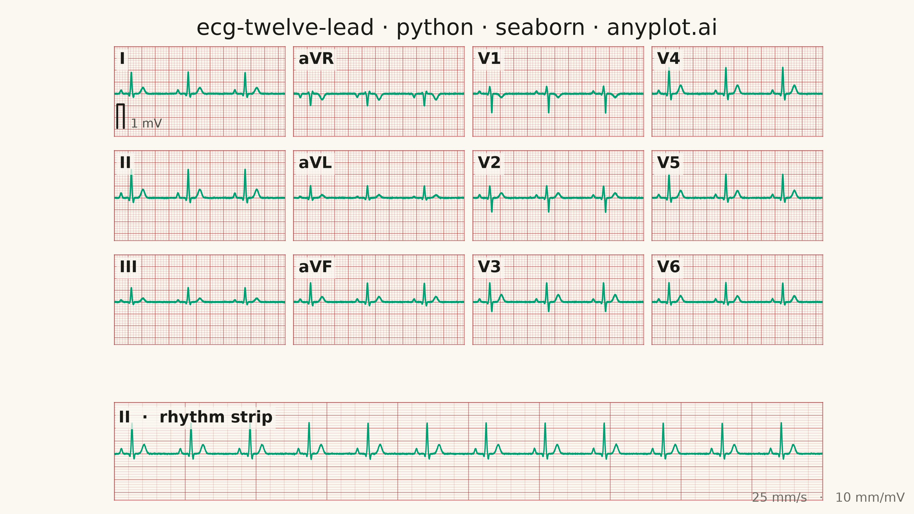
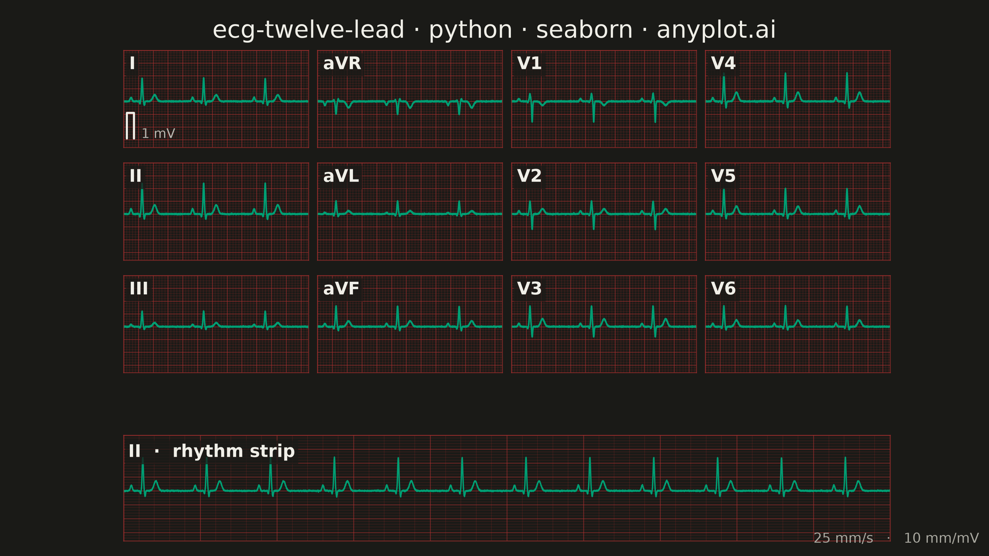
A multi-channel electrocardiogram display showing the 12 standard ECG leads arranged in clinical format. Each lead displays realistic P-QRS-T wave complexes on a medical-standard grid background with calibration markers. This visualization replicates the familiar layout used in hospitals and clinics worldwide, making it immediately recognizable to healthcare professionals and useful for medical education.
""" anyplot.ai
ecg-twelve-lead: ECG/EKG 12-Lead Waveform Display
Library: seaborn 0.13.2 | Python 3.13.14
Quality: 93/100 | Updated: 2026-06-17
"""

import os

import matplotlib.pyplot as plt
import matplotlib.ticker as ticker
import numpy as np
import pandas as pd
import seaborn as sns
import seaborn.objects as so


# Theme-adaptive chrome (Imprint)
THEME = os.getenv("ANYPLOT_THEME", "light")
PAGE_BG = "#FAF8F1" if THEME == "light" else "#1A1A17"
INK = "#1A1A17" if THEME == "light" else "#F0EFE8"
INK_SOFT = "#4A4A44" if THEME == "light" else "#B8B7B0"
INK_MUTED = "#6B6A63" if THEME == "light" else "#A8A79F"

# Imprint palette: the ECG trace is the single data series, so it takes the brand
# green (#009E73) — also the classic green-on-monitor cardiac look. The iconic ECG
# paper grid uses the matte-red medical/blood semantic anchor (#AE3030).
BRAND = "#009E73"
GRID_RED = "#AE3030"
grid_major_alpha = 0.50 if THEME == "light" else 0.55
grid_minor_alpha = 0.20 if THEME == "light" else 0.24

sns.set_theme(
    style="white",
    rc={
        "figure.facecolor": PAGE_BG,
        "axes.facecolor": PAGE_BG,
        "text.color": INK,
        "axes.labelcolor": INK,
        "xtick.color": INK_SOFT,
        "ytick.color": INK_SOFT,
    },
)

# Data - synthetic normal sinus rhythm via a Gaussian P-QRS-T wave model, emitted
# into one long-form (tidy) DataFrame so seaborn can facet the 12 leads natively.
np.random.seed(42)
sampling_rate = 1000
duration = 2.5
time = np.linspace(0, duration, int(sampling_rate * duration))
heart_rate = 72
rr_interval = 60.0 / heart_rate

wave_centers = np.array([0.10, 0.22, 0.25, 0.28, 0.42])
wave_widths = np.array([0.012, 0.005, 0.008, 0.006, 0.025])
wave_keys = ["p", "q", "r", "s", "t"]

lead_configs = {
    "I": {"p": 0.15, "q": -0.08, "r": 0.9, "s": -0.15, "t": 0.25},
    "II": {"p": 0.20, "q": -0.10, "r": 1.2, "s": -0.20, "t": 0.35},
    "III": {"p": 0.08, "q": -0.05, "r": 0.6, "s": -0.10, "t": 0.15},
    "aVR": {"p": -0.15, "q": 0.05, "r": -0.5, "s": 0.10, "t": -0.25},
    "aVL": {"p": 0.05, "q": -0.06, "r": 0.5, "s": -0.08, "t": 0.12},
    "aVF": {"p": 0.12, "q": -0.08, "r": 0.8, "s": -0.15, "t": 0.22},
    "V1": {"p": 0.10, "q": -0.04, "r": 0.3, "s": -0.8, "t": -0.15},
    "V2": {"p": 0.12, "q": -0.05, "r": 0.5, "s": -0.6, "t": 0.20},
    "V3": {"p": 0.12, "q": -0.06, "r": 0.8, "s": -0.4, "t": 0.30},
    "V4": {"p": 0.14, "q": -0.08, "r": 1.1, "s": -0.25, "t": 0.35},
    "V5": {"p": 0.14, "q": -0.08, "r": 1.0, "s": -0.18, "t": 0.30},
    "V6": {"p": 0.12, "q": -0.06, "r": 0.8, "s": -0.12, "t": 0.25},
}


def synth_ecg(t, gains):
    """Sum Gaussian P-Q-R-S-T waves across every beat in the window, add fine noise."""
    signal = np.zeros_like(t)
    gain_values = np.array([gains[k] for k in wave_keys])
    for beat_start in np.arange(0, t[-1] + rr_interval, rr_interval):
        dt = t - beat_start
        for i in range(5):
            signal += gain_values[i] * np.exp(-((dt - wave_centers[i]) ** 2) / (2 * wave_widths[i] ** 2))
    return signal + np.random.normal(0, 0.01, len(t))


def style_ecg_grid(ax, xmax, x_major, x_minor):
    """Render an axis as standard ECG paper: major/minor red grid, no ticks, framed."""
    ax.set_xlim(0, xmax)
    ax.set_ylim(-1.8, 2.0)
    ax.set_title("")
    ax.xaxis.set_major_locator(ticker.MultipleLocator(x_major))
    ax.xaxis.set_minor_locator(ticker.MultipleLocator(x_minor))
    ax.yaxis.set_major_locator(ticker.MultipleLocator(0.5))
    ax.yaxis.set_minor_locator(ticker.MultipleLocator(0.1))
    ax.grid(which="major", color=GRID_RED, alpha=grid_major_alpha, linewidth=0.5)
    ax.grid(which="minor", color=GRID_RED, alpha=grid_minor_alpha, linewidth=0.3)
    ax.set_facecolor(PAGE_BG)
    ax.set_xticklabels([])
    ax.set_yticklabels([])
    ax.set_xlabel("")
    ax.set_ylabel("")
    ax.tick_params(axis="both", which="both", length=0)
    for spine in ax.spines.values():
        spine.set_color(GRID_RED)
        spine.set_alpha(grid_major_alpha)
        spine.set_linewidth(0.6)


# Clinical 3x4 lead order + a full-length Lead II rhythm strip below.
lead_order = ["I", "aVR", "V1", "V4", "II", "aVL", "V2", "V5", "III", "aVF", "V3", "V6"]
leads_df = pd.concat(
    [pd.DataFrame({"time": time, "voltage": synth_ecg(time, lead_configs[lead]), "lead": lead}) for lead in lead_order],
    ignore_index=True,
)
leads_df["lead"] = pd.Categorical(leads_df["lead"], categories=lead_order, ordered=True)

rhythm_duration = duration * 4
rhythm_time = np.linspace(0, rhythm_duration, int(sampling_rate * rhythm_duration))
rhythm_df = pd.DataFrame({"time": rhythm_time, "voltage": synth_ecg(rhythm_time, lead_configs["II"])})

# Plot - exact 3200x1800 canvas; an outer gridspec carves a 3x4 facet block and a
# full-width rhythm strip into two subfigures, each drawn by the seaborn objects API.
fig = plt.figure(figsize=(8, 4.5), dpi=400)
fig.set_facecolor(PAGE_BG)
outer = fig.add_gridspec(2, 1, height_ratios=[3.05, 1.0], left=0.025, right=0.99, top=0.905, bottom=0.06, hspace=0.10)
sf_leads = fig.add_subfigure(outer[0])
sf_rhythm = fig.add_subfigure(outer[1])
sf_leads.set_facecolor(PAGE_BG)
sf_rhythm.set_facecolor(PAGE_BG)

# 12 leads as a native seaborn facet grid via the objects interface.
(
    so.Plot(leads_df, x="time", y="voltage")
    .facet(col="lead", order=lead_order, wrap=4)
    .add(so.Line(color=BRAND, linewidth=0.9))
    .limit(x=(0, duration), y=(-1.8, 2.0))
    .label(x="", y="", title="")
    .share(x=True, y=True)
    .on(sf_leads)
    .plot()
)

label_bbox = {"boxstyle": "square,pad=0.18", "facecolor": PAGE_BG, "edgecolor": "none", "alpha": 0.75}
sf_leads.subplots_adjust(wspace=0.05, hspace=0.16)
for ax, lead in zip(sf_leads.axes, lead_order, strict=True):
    style_ecg_grid(ax, duration, 0.2, 0.04)
    ax.text(
        0.03,
        0.94,
        lead,
        transform=ax.transAxes,
        fontsize=10,
        fontweight="bold",
        color=INK,
        va="top",
        zorder=10,
        bbox=label_bbox,
    )

# 1 mV calibration pulse in the first panel, parked low-left clear of the trace.
cal_ax = sf_leads.axes[0]
cal_x0, cal_w = 0.04, 0.10
cal_ax.plot(
    [cal_x0, cal_x0, cal_x0 + cal_w, cal_x0 + cal_w], [-1.45, -0.45, -0.45, -1.45], color=INK, linewidth=1.2, zorder=8
)
cal_ax.text(cal_x0 + cal_w + 0.10, -1.30, "1 mV", fontsize=7.5, ha="left", va="center", color=INK_SOFT)

# Rhythm strip - Lead II running across the full width, also drawn by the objects API.
ax_rhythm = sf_rhythm.subplots()
(
    so.Plot(rhythm_df, x="time", y="voltage")
    .add(so.Line(color=BRAND, linewidth=0.8))
    .limit(x=(0, rhythm_duration), y=(-1.8, 2.0))
    .label(x="", y="")
    .on(ax_rhythm)
    .plot()
)
style_ecg_grid(ax_rhythm, rhythm_duration, 1.0, 0.2)
ax_rhythm.text(
    0.006,
    0.92,
    "II  ·  rhythm strip",
    transform=ax_rhythm.transAxes,
    fontsize=10,
    fontweight="bold",
    color=INK,
    va="top",
    zorder=10,
    bbox=label_bbox,
)

# Title and scale footer
fig.suptitle("ecg-twelve-lead · python · seaborn · anyplot.ai", fontsize=14, fontweight="medium", color=INK, y=0.965)
fig.text(0.99, 0.018, "25 mm/s   ·   10 mm/mV", fontsize=8, ha="right", va="bottom", color=INK_MUTED)

# Save - exact 3200x1800 (8x4.5 in @ 400 dpi); no bbox_inches so canvas stays on target
fig.savefig(f"plot-{THEME}.png", dpi=400, facecolor=PAGE_BG)
Runnable source as JSON, for any HTTP client: https://api.anyplot.ai/specs/ecg-twelve-lead/seaborn/code. Any spec id and library id listed in llms-full.txt fit the same URL shape; every URL below is complete and callable.
{
  "spec_id": "ecg-twelve-lead",
  "language": "python",
  "library": "seaborn",
  "page": "https://anyplot.ai/ecg-twelve-lead/python/seaborn",
  "hub": "https://anyplot.ai/ecg-twelve-lead",
  "code_json": "https://api.anyplot.ai/specs/ecg-twelve-lead/seaborn/code",
  "spec_json": "https://api.anyplot.ai/specs/ecg-twelve-lead",
  "render_light_png": "https://storage.googleapis.com/anyplot-images/plots/ecg-twelve-lead/python/seaborn/plot-light.png",
  "render_dark_png": "https://storage.googleapis.com/anyplot-images/plots/ecg-twelve-lead/python/seaborn/plot-dark.png",
  "quality_score": 93.0,
  "license": "MIT",
  "guide": "https://anyplot.ai/llms.txt"
}
Part of ECG/EKG 12-Lead Waveform Display on anyplot.ai.