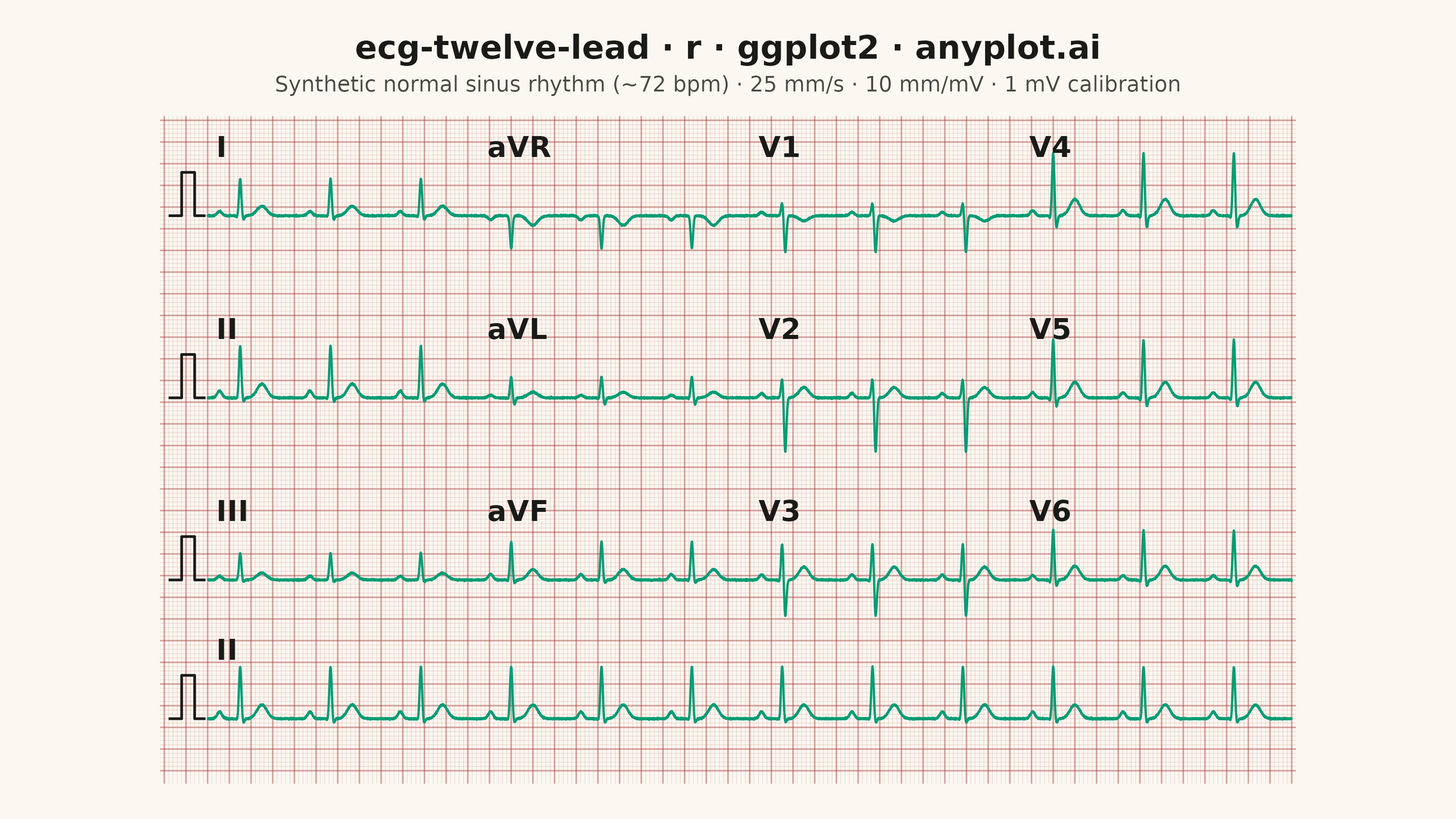
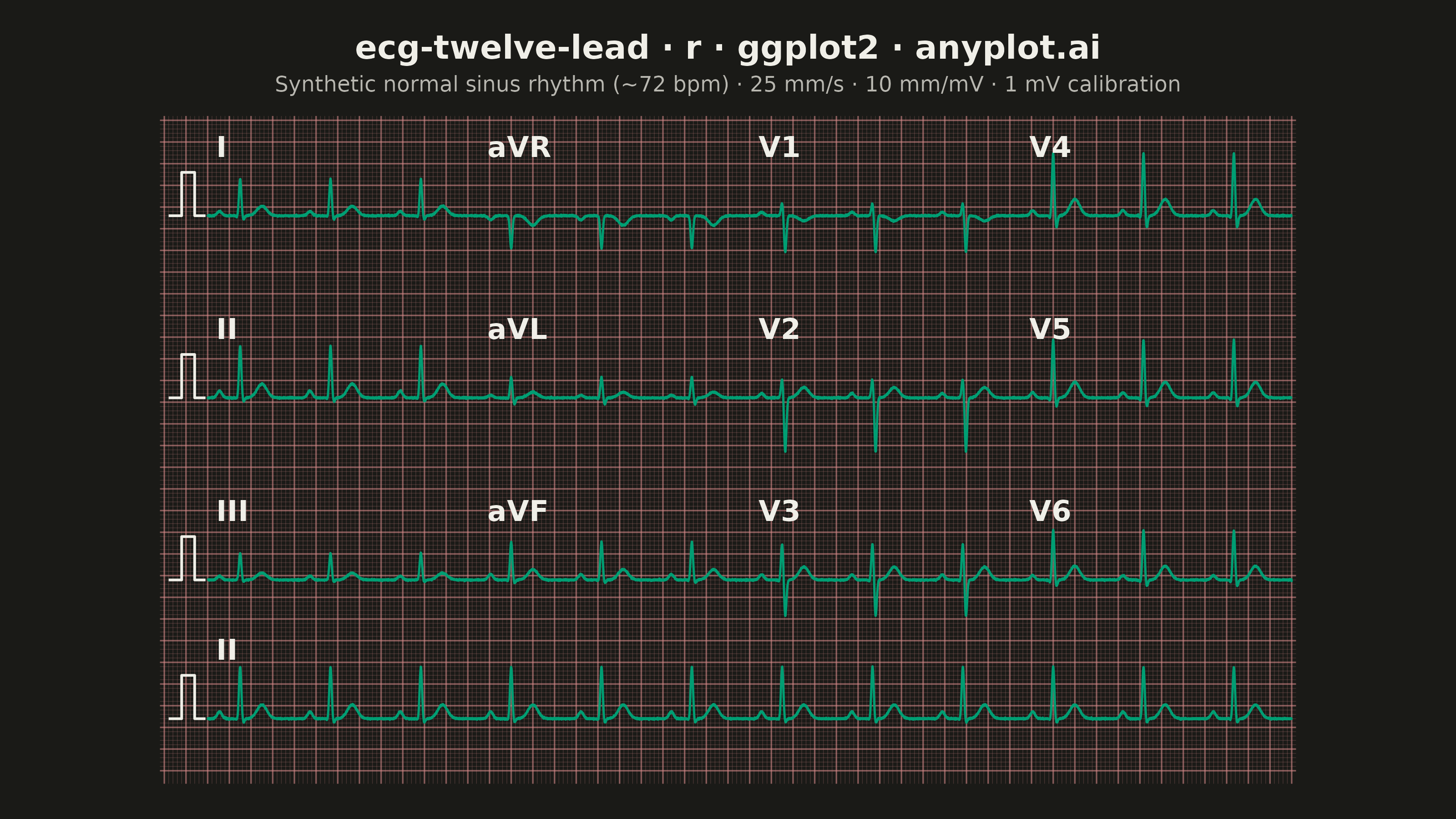
A multi-channel electrocardiogram display showing the 12 standard ECG leads arranged in clinical format. Each lead displays realistic P-QRS-T wave complexes on a medical-standard grid background with calibration markers. This visualization replicates the familiar layout used in hospitals and clinics worldwide, making it immediately recognizable to healthcare professionals and useful for medical education.
#' anyplot.ai
#' ecg-twelve-lead: ECG/EKG 12-Lead Waveform Display
#' Library: ggplot2 3.5.1 | R 4.4.1
#' Quality: 93/100 | Created: 2026-06-17

library(ggplot2)
library(dplyr)
library(ragg)

set.seed(42)

# --- Theme tokens -----------------------------------------------------------
THEME    <- Sys.getenv("ANYPLOT_THEME", "light")
PAGE_BG  <- if (THEME == "light") "#FAF8F1" else "#1A1A17"
INK      <- if (THEME == "light") "#1A1A17" else "#F0EFE8"
INK_SOFT <- if (THEME == "light") "#4A4A44" else "#B8B7B0"

# Imprint palette — first series is always brand green; the ECG trace is the
# single data series, so it renders in position 1 (#009E73).
TRACE <- "#009E73"

# ECG paper grid uses the classic medical red/pink, derived from the Imprint
# matte-red anchor (#AE3030). Lighter on the dark surface so it stays visible.
GRID_COL    <- if (THEME == "light") "#AE3030" else "#D98C8C"
MINOR_ALPHA <- if (THEME == "light") 0.16 else 0.24
MAJOR_ALPHA <- if (THEME == "light") 0.38 else 0.50

# --- ECG model --------------------------------------------------------------
# Standard scale: 25 mm/s (time) and 10 mm/mV (voltage). We work in millimetre
# coordinates so that one small grid box (1 mm) equals 0.04 s and 0.1 mV, and
# coord_fixed keeps the boxes square — the authentic ECG-paper look.
MM_PER_S  <- 25      # horizontal calibration
MM_PER_MV <- 10      # vertical calibration
RR        <- 60 / 72 # normal sinus rhythm, ~72 bpm

# Single-beat P-QRS-T morphology built from Gaussian components. The phase
# wraps with the RR interval so every beat in a strip is identical.
strip_t <- seq(0, 2.5, length.out = 2500)   # 2.5 s per cell at 1000 Hz
strip_ph <- ((strip_t - 0.30 + RR / 2) %% RR) - RR / 2

# Per-lead wave amplitudes (mV) reproduce normal precordial/limb morphology:
# rS pattern in V1-V2, tall R in V4-V6, fully inverted aVR, etc.
leads <- tibble::tribble(
    ~lead, ~row, ~col, ~p, ~q, ~r, ~s, ~tw,
    "I", 1L, 1L, 0.10, -0.04, 0.85, -0.10, 0.22,
    "aVR", 1L, 2L, -0.10, 0.00, -0.75, 0.00, -0.22,
    "V1", 1L, 3L, 0.08, 0.00, 0.30, -0.85, -0.12,
    "V4", 1L, 4L, 0.12, -0.08, 1.45, -0.30, 0.38,
    "II", 2L, 1L, 0.16, -0.04, 1.20, -0.10, 0.32,
    "aVL", 2L, 2L, 0.06, -0.03, 0.48, -0.16, 0.13,
    "V2", 2L, 3L, 0.10, 0.00, 0.45, -1.25, 0.24,
    "V5", 2L, 4L, 0.12, -0.10, 1.35, -0.22, 0.36,
    "III", 3L, 1L, 0.09, 0.00, 0.62, -0.05, 0.16,
    "aVF", 3L, 2L, 0.13, -0.03, 0.88, -0.08, 0.24,
    "V3", 3L, 3L, 0.12, -0.05, 0.85, -0.85, 0.30,
    "V6", 3L, 4L, 0.10, -0.08, 1.15, -0.16, 0.32
)

row_center <- c(128, 86, 44)        # mm, top row highest
col_x <- function(c) (c - 1) * (2.5 * MM_PER_S)  # 62.5 mm per cell

# Build the 12 lead strips into one long data frame.
strip_list <- vector("list", nrow(leads))
for (i in seq_len(nrow(leads))) {
    lp <- leads[i, ]
    wave <- lp$p * exp(-0.5 * ((strip_ph + 0.190) / 0.022)^2) +
        lp$q * exp(-0.5 * ((strip_ph + 0.025) / 0.0085)^2) +
        lp$r * exp(-0.5 * ((strip_ph + 0.000) / 0.011)^2) +
        lp$s * exp(-0.5 * ((strip_ph - 0.028) / 0.011)^2) +
        lp$tw * exp(-0.5 * ((strip_ph - 0.200) / 0.045)^2)
    wave <- wave + rnorm(length(strip_t), 0, 0.008)
    strip_list[[i]] <- tibble::tibble(
        x = col_x(lp$col) + strip_t * MM_PER_S,
        y = row_center[lp$row] + wave * MM_PER_MV,
        lead = lp$lead
    )
}
ecg <- bind_rows(strip_list)

# Full-length Lead II rhythm strip across the bottom (10 s continuous).
rhythm_t <- seq(0, 10, length.out = 10000)
rhythm_ph <- ((rhythm_t - 0.30 + RR / 2) %% RR) - RR / 2
rhythm_wave <- 0.16 * exp(-0.5 * ((rhythm_ph + 0.190) / 0.022)^2) +
    -0.04 * exp(-0.5 * ((rhythm_ph + 0.025) / 0.0085)^2) +
    1.20 * exp(-0.5 * ((rhythm_ph + 0.000) / 0.011)^2) +
    -0.10 * exp(-0.5 * ((rhythm_ph - 0.028) / 0.011)^2) +
    0.32 * exp(-0.5 * ((rhythm_ph - 0.200) / 0.045)^2)
rhythm_wave <- rhythm_wave + rnorm(length(rhythm_t), 0, 0.008)
rhythm <- tibble::tibble(
    x = rhythm_t * MM_PER_S,
    y = 12 + rhythm_wave * MM_PER_MV,
    lead = "II"
)

# 1 mV calibration pulses (a 10 mm step) at the left margin of every row.
cal_centers <- c(row_center, 12)
cal_list <- vector("list", length(cal_centers))
for (i in seq_along(cal_centers)) {
    cal_list[[i]] <- tibble::tibble(
        x = c(-9, -6, -6, -3, -3, -0.5),
        y = cal_centers[i] + c(0, 0, 10, 10, 0, 0),
        grp = i
    )
}
cal <- bind_rows(cal_list)

# Lead name labels at the top-left of each cell.
labels <- tibble::tibble(
    x = col_x(leads$col) + 2,
    y = row_center[leads$row] + 16,
    lead = leads$lead
)
labels <- bind_rows(labels, tibble::tibble(x = 2, y = 12 + 16, lead = "II"))

# Grid coordinates (1 mm minor, 5 mm major) spanning the full display.
x_lo <- -11
x_hi <- 251
y_lo <- -3
y_hi <- 151
minor_x <- seq(-10, 250, by = 1)
minor_y <- seq(0, 150, by = 1)
major_x <- seq(-10, 250, by = 5)
major_y <- seq(0, 150, by = 5)

# --- Plot -------------------------------------------------------------------
p <- ggplot() +
    geom_vline(xintercept = minor_x, color = GRID_COL, linewidth = 0.12, alpha = MINOR_ALPHA) +
    geom_hline(yintercept = minor_y, color = GRID_COL, linewidth = 0.12, alpha = MINOR_ALPHA) +
    geom_vline(xintercept = major_x, color = GRID_COL, linewidth = 0.30, alpha = MAJOR_ALPHA) +
    geom_hline(yintercept = major_y, color = GRID_COL, linewidth = 0.30, alpha = MAJOR_ALPHA) +
    geom_path(data = cal, aes(x = x, y = y, group = grp), color = INK, linewidth = 0.5) +
    geom_path(data = ecg, aes(x = x, y = y, group = lead), color = TRACE, linewidth = 0.42) +
    geom_path(data = rhythm, aes(x = x, y = y), color = TRACE, linewidth = 0.42) +
    geom_text(
        data = labels, aes(x = x, y = y, label = lead),
        color = INK, fontface = "bold", size = 4, hjust = 0
    ) +
    labs(
        title = "ecg-twelve-lead · r · ggplot2 · anyplot.ai",
        subtitle = "Synthetic normal sinus rhythm (~72 bpm) · 25 mm/s · 10 mm/mV · 1 mV calibration"
    ) +
    coord_fixed(ratio = 1, xlim = c(x_lo, x_hi), ylim = c(y_lo, y_hi), expand = FALSE) +
    theme_void(base_size = 8) +
    theme(
        plot.background = element_rect(fill = PAGE_BG, color = PAGE_BG),
        panel.background = element_rect(fill = PAGE_BG, color = NA),
        plot.title = element_text(color = INK, size = 13, face = "bold", hjust = 0.5,
                                  margin = margin(b = 4)),
        plot.subtitle = element_text(color = INK_SOFT, size = 8.5, hjust = 0.5,
                                     margin = margin(b = 8)),
        plot.margin = margin(14, 18, 14, 18)
    )

# --- Save -------------------------------------------------------------------
ggsave(
    filename = sprintf("plot-%s.png", THEME),
    plot = p,
    device = ragg::agg_png,
    width = 8,
    height = 4.5,
    units = "in",
    dpi = 400
)
Runnable source as JSON, for any HTTP client: https://api.anyplot.ai/specs/ecg-twelve-lead/ggplot2/code. Any spec id and library id listed in llms-full.txt fit the same URL shape; every URL below is complete and callable.
{
  "spec_id": "ecg-twelve-lead",
  "language": "r",
  "library": "ggplot2",
  "page": "https://anyplot.ai/ecg-twelve-lead/r/ggplot2",
  "hub": "https://anyplot.ai/ecg-twelve-lead",
  "code_json": "https://api.anyplot.ai/specs/ecg-twelve-lead/ggplot2/code",
  "spec_json": "https://api.anyplot.ai/specs/ecg-twelve-lead",
  "render_light_png": "https://storage.googleapis.com/anyplot-images/plots/ecg-twelve-lead/r/ggplot2/plot-light.png",
  "render_dark_png": "https://storage.googleapis.com/anyplot-images/plots/ecg-twelve-lead/r/ggplot2/plot-dark.png",
  "quality_score": 93.0,
  "license": "MIT",
  "guide": "https://anyplot.ai/llms.txt"
}
Part of ECG/EKG 12-Lead Waveform Display on anyplot.ai.