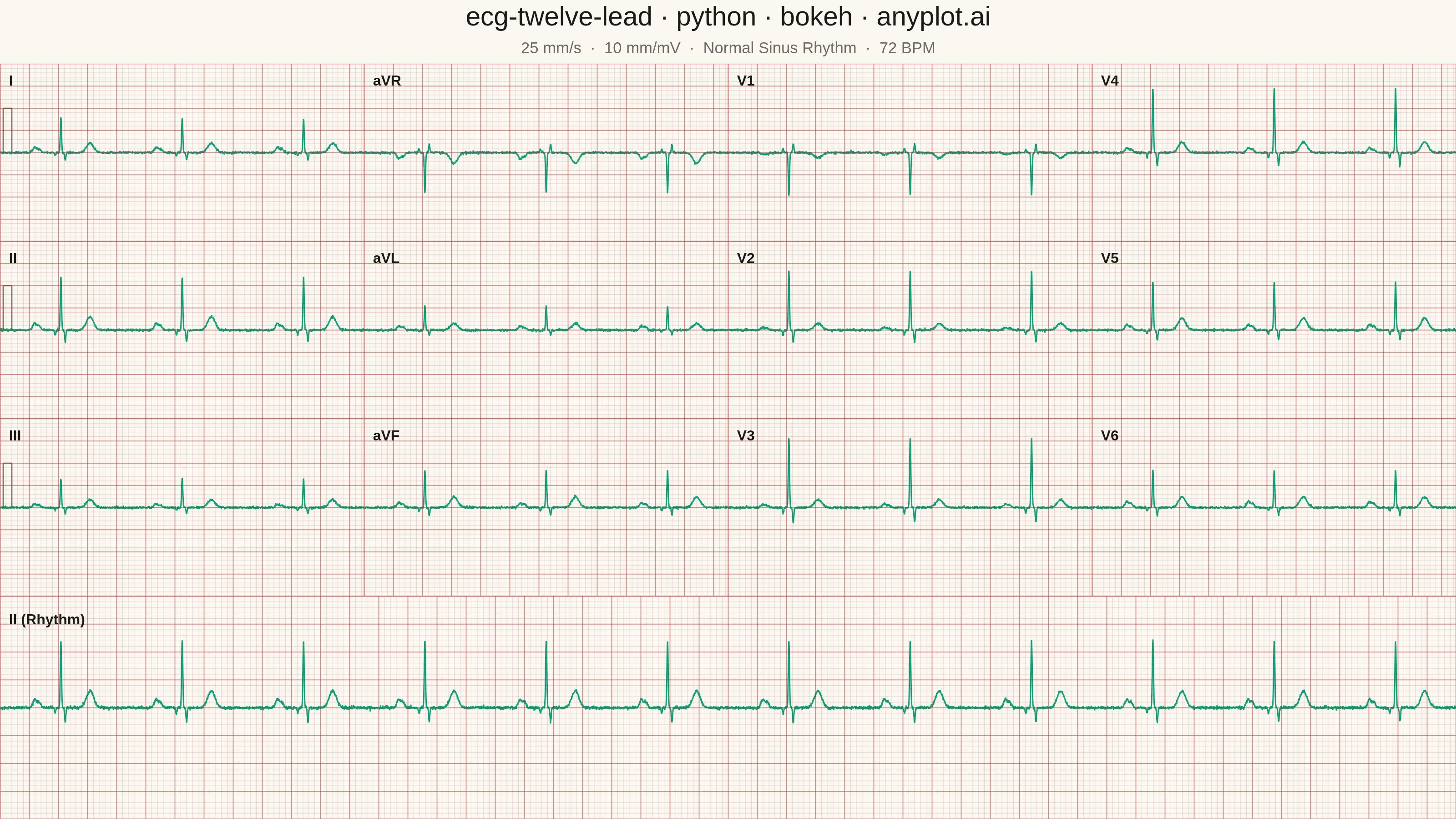
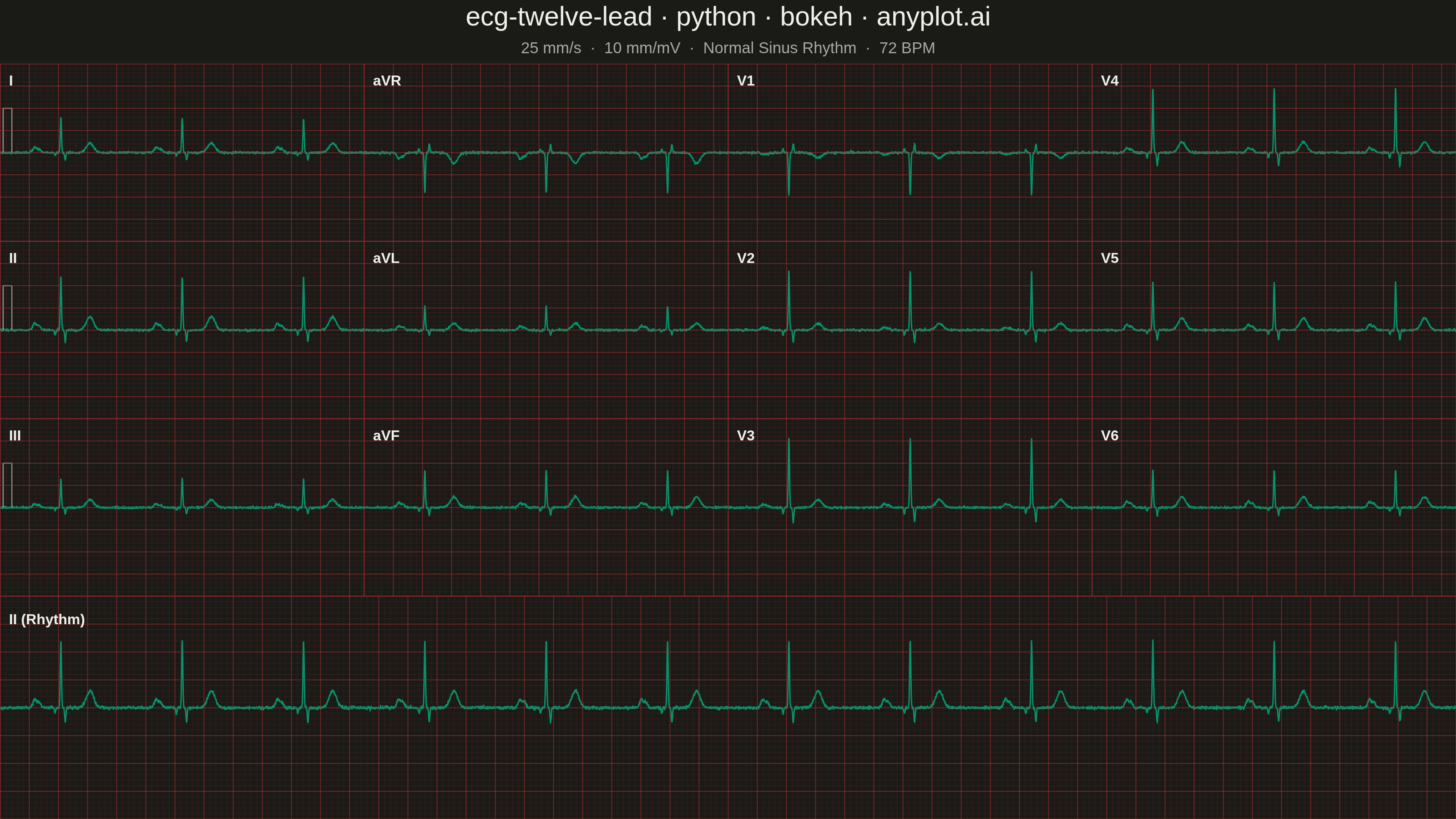
A multi-channel electrocardiogram display showing the 12 standard ECG leads arranged in clinical format. Each lead displays realistic P-QRS-T wave complexes on a medical-standard grid background with calibration markers. This visualization replicates the familiar layout used in hospitals and clinics worldwide, making it immediately recognizable to healthcare professionals and useful for medical education.
""" anyplot.ai
ecg-twelve-lead: ECG/EKG 12-Lead Waveform Display
Library: bokeh 3.9.1 | Python 3.13.14
Quality: 92/100 | Updated: 2026-06-17
"""

import os
import time
from pathlib import Path

import numpy as np
from bokeh.io import output_file, save
from bokeh.layouts import column, gridplot
from bokeh.models import ColumnDataSource, HoverTool, Label, Range1d, Span
from bokeh.plotting import figure
from selenium import webdriver
from selenium.webdriver.chrome.options import Options


# Theme-adaptive chrome (Imprint palette)
THEME = os.getenv("ANYPLOT_THEME", "light")
PAGE_BG = "#FAF8F1" if THEME == "light" else "#1A1A17"
INK = "#1A1A17" if THEME == "light" else "#F0EFE8"
INK_SOFT = "#4A4A44" if THEME == "light" else "#B8B7B0"
INK_MUTED = "#6B6A63" if THEME == "light" else "#A8A79F"

# Imprint palette — brand green is the single ECG trace (position 1, always first).
# The ECG-paper look comes from a red ruling (Imprint matte red #AE3030) over the
# theme background instead of a custom pink paper fill, keeping the brand surface.
TRACE_COLOR = "#009E73"
ECG_RED = "#AE3030"
grid_major_alpha = 0.45 if THEME == "light" else 0.50
grid_minor_alpha = 0.18 if THEME == "light" else 0.22

# Data - Synthetic ECG waveform generation using Gaussian pulse model
np.random.seed(42)

sampling_rate = 1000
duration = 2.5
n_samples = int(sampling_rate * duration)
t = np.linspace(0, duration, n_samples)

heart_rate_bpm = 72
beat_interval = 60.0 / heart_rate_bpm
beat_centers = np.arange(beat_interval / 2, duration, beat_interval)

# Gaussian pulse parameters: (center_offset, sigma, amplitude)
p_wave_params = [(-0.18, 0.012, 0.15), (-0.15, 0.012, 0.10)]
qrs_params = [(-0.04, 0.004, -0.10), (0.0, 0.004, 1.20), (0.03, 0.004, -0.25)]
t_wave_params = [(0.20, 0.025, 0.30)]

# Lead transformation factors (approximate Einthoven/Goldberger/Wilson relations)
lead_transforms = {
    "I": {"scale": 0.65, "invert": False, "p_scale": 0.8, "t_scale": 0.7},
    "II": {"scale": 1.0, "invert": False, "p_scale": 1.0, "t_scale": 1.0},
    "III": {"scale": 0.55, "invert": False, "p_scale": 0.5, "t_scale": 0.6},
    "aVR": {"scale": 0.75, "invert": True, "p_scale": 0.9, "t_scale": 0.8},
    "aVL": {"scale": 0.45, "invert": False, "p_scale": 0.6, "t_scale": 0.5},
    "aVF": {"scale": 0.70, "invert": False, "p_scale": 0.7, "t_scale": 0.8},
    "V1": {"scale": 0.80, "invert": True, "p_scale": 0.3, "t_scale": 0.4},
    "V2": {"scale": 1.10, "invert": False, "p_scale": 0.4, "t_scale": 0.5},
    "V3": {"scale": 1.30, "invert": False, "p_scale": 0.5, "t_scale": 0.6},
    "V4": {"scale": 1.20, "invert": False, "p_scale": 0.7, "t_scale": 0.8},
    "V5": {"scale": 0.90, "invert": False, "p_scale": 0.8, "t_scale": 0.9},
    "V6": {"scale": 0.70, "invert": False, "p_scale": 0.9, "t_scale": 0.8},
}


def synth_beat(t_axis, centers, params):
    """Sum Gaussian P-QRS-T complexes at each beat center for one lead."""
    signal = np.zeros(len(t_axis))
    for center in centers:
        t_shifted = t_axis - center
        for offset, sigma, amp in p_wave_params:
            signal += amp * params["p_scale"] * np.exp(-((t_shifted - offset) ** 2) / (2 * sigma**2))
        for offset, sigma, amp in qrs_params:
            signal += amp * params["scale"] * np.exp(-((t_shifted - offset) ** 2) / (2 * sigma**2))
        for offset, sigma, amp in t_wave_params:
            signal += amp * params["t_scale"] * np.exp(-((t_shifted - offset) ** 2) / (2 * sigma**2))
    if params["invert"]:
        signal = -signal
    return signal + np.random.normal(0, 0.015, len(t_axis))


leads = {name: synth_beat(t, beat_centers, params) for name, params in lead_transforms.items()}

# Standard clinical 3x4 grid layout
grid_layout = [["I", "aVR", "V1", "V4"], ["II", "aVL", "V2", "V5"], ["III", "aVF", "V3", "V6"]]

# Plot - canvas is a fixed 3200x1800: title band (140) + 3x4 grid (3*390) + rhythm strip (490)
panel_w = 800  # 4 columns * 800 = 3200
panel_h = 390  # 3 rows * 390 = 1170
title_h = 140
rhythm_h = 490
y_range_mv = 2.0


def add_ecg_grid(p, x_max, y_min, y_max):
    """Draw ECG-paper ruling: bold lines every 5mm (0.2s / 0.5mV), fine every 1mm."""
    for x_major in np.arange(0, x_max + 0.01, 0.2):
        p.add_layout(
            Span(location=x_major, dimension="height", line_color=ECG_RED, line_width=2, line_alpha=grid_major_alpha)
        )
    for y_major in np.arange(y_min, y_max + 0.01, 0.5):
        p.add_layout(
            Span(location=y_major, dimension="width", line_color=ECG_RED, line_width=2, line_alpha=grid_major_alpha)
        )
    for x_minor in np.arange(0, x_max + 0.01, 0.04):
        p.add_layout(
            Span(location=x_minor, dimension="height", line_color=ECG_RED, line_width=1, line_alpha=grid_minor_alpha)
        )
    for y_minor in np.arange(y_min, y_max + 0.01, 0.1):
        p.add_layout(
            Span(location=y_minor, dimension="width", line_color=ECG_RED, line_width=1, line_alpha=grid_minor_alpha)
        )


def style_ecg_panel(p):
    """Apply common ECG panel styling (hidden axes, theme surface)."""
    p.xaxis.visible = False
    p.yaxis.visible = False
    p.xgrid.grid_line_color = None
    p.ygrid.grid_line_color = None
    p.background_fill_color = PAGE_BG
    p.border_fill_color = PAGE_BG
    p.outline_line_color = ECG_RED
    p.outline_line_width = 1
    p.outline_line_alpha = grid_major_alpha
    p.min_border = 0


def draw_trace(p, t_axis, signal, label):
    """Add the ECG trace, hover readout, and lead label to a panel."""
    source = ColumnDataSource(data={"time": t_axis, "voltage": signal})
    line = p.line(x="time", y="voltage", source=source, line_color=TRACE_COLOR, line_width=3.0, line_alpha=0.95)
    p.add_tools(
        HoverTool(
            renderers=[line],
            tooltips=[("Lead", label), ("t", "@time{0.000} s"), ("mV", "@voltage{0.00}")],
            mode="vline",
        )
    )
    p.add_layout(
        Label(x=0.06, y=y_range_mv * 0.72, text=label, text_font_size="24pt", text_font_style="bold", text_color=INK)
    )


figures = []
for lead_row in grid_layout:
    fig_row = []
    for col_idx, lead_name in enumerate(lead_row):
        p = figure(
            width=panel_w,
            height=panel_h,
            x_range=Range1d(0, duration),
            y_range=Range1d(-y_range_mv, y_range_mv),
            toolbar_location=None,
        )
        add_ecg_grid(p, duration, -y_range_mv, y_range_mv)
        draw_trace(p, t, leads[lead_name], lead_name)

        # 1mV calibration pulse at the start of the leftmost column
        if col_idx == 0:
            p.line(
                x=[0.02, 0.02, 0.08, 0.08], y=[0.0, 1.0, 1.0, 0.0], line_color=INK_SOFT, line_width=2.5, line_alpha=0.8
            )

        style_ecg_panel(p)
        fig_row.append(p)
    figures.append(fig_row)

# Rhythm strip (Lead II, 10 seconds)
rhythm_duration = 10.0
rhythm_t = np.linspace(0, rhythm_duration, int(sampling_rate * rhythm_duration))
rhythm_centers = np.arange(beat_interval / 2, rhythm_duration, beat_interval)
rhythm_signal = synth_beat(rhythm_t, rhythm_centers, lead_transforms["II"])

p_rhythm = figure(
    width=panel_w * 4,
    height=rhythm_h,
    x_range=Range1d(0, rhythm_duration),
    y_range=Range1d(-y_range_mv, y_range_mv),
    toolbar_location=None,
)
add_ecg_grid(p_rhythm, rhythm_duration, -y_range_mv, y_range_mv)
draw_trace(p_rhythm, rhythm_t, rhythm_signal, "II (Rhythm)")
style_ecg_panel(p_rhythm)

# Title band
p_title = figure(width=panel_w * 4, height=title_h, toolbar_location=None, x_range=Range1d(0, 1), y_range=Range1d(0, 1))
p_title.add_layout(
    Label(
        x=0.5,
        y=0.52,
        text="ecg-twelve-lead · python · bokeh · anyplot.ai",
        text_font_size="44pt",
        text_color=INK,
        text_align="center",
    )
)
p_title.add_layout(
    Label(
        x=0.5,
        y=0.12,
        text="25 mm/s  ·  10 mm/mV  ·  Normal Sinus Rhythm  ·  72 BPM",
        text_font_size="26pt",
        text_color=INK_MUTED,
        text_align="center",
    )
)
p_title.xaxis.visible = False
p_title.yaxis.visible = False
p_title.xgrid.grid_line_color = None
p_title.ygrid.grid_line_color = None
p_title.background_fill_color = PAGE_BG
p_title.border_fill_color = PAGE_BG
p_title.outline_line_color = None
p_title.min_border = 0

# Assemble layout (total 3200x1800)
grid = gridplot(figures, toolbar_location=None, merge_tools=False)
layout = column(p_title, grid, p_rhythm, spacing=0, background=PAGE_BG)

# Save — HTML artifact, then screenshot it with headless Chrome (export_png is unreliable here)
output_file(f"plot-{THEME}.html", title="ecg-twelve-lead · python · bokeh · anyplot.ai")
save(layout)

W, H = 3200, 1800
opts = Options()
for arg in (
    "--headless=new",
    "--no-sandbox",
    "--disable-dev-shm-usage",
    "--disable-gpu",
    f"--window-size={W},{H}",
    "--hide-scrollbars",
):
    opts.add_argument(arg)
driver = webdriver.Chrome(options=opts)
# Force the rendering viewport to exactly W x H — headless Chrome's window chrome
# otherwise shrinks the captured viewport (3200x1800 window -> ~3200x1657 screenshot).
driver.execute_cdp_cmd(
    "Emulation.setDeviceMetricsOverride", {"width": W, "height": H, "deviceScaleFactor": 1, "mobile": False}
)
driver.get(f"file://{Path(f'plot-{THEME}.html').resolve()}")
time.sleep(3)  # let bokeh's JS render the canvas
driver.execute_script(f"document.body.style.margin='0';document.documentElement.style.background='{PAGE_BG}';")
time.sleep(0.3)
driver.save_screenshot(f"plot-{THEME}.png")
driver.quit()
Runnable source as JSON, for any HTTP client: https://api.anyplot.ai/specs/ecg-twelve-lead/bokeh/code. Any spec id and library id listed in llms-full.txt fit the same URL shape; every URL below is complete and callable.
{
  "spec_id": "ecg-twelve-lead",
  "language": "python",
  "library": "bokeh",
  "page": "https://anyplot.ai/ecg-twelve-lead/python/bokeh",
  "hub": "https://anyplot.ai/ecg-twelve-lead",
  "code_json": "https://api.anyplot.ai/specs/ecg-twelve-lead/bokeh/code",
  "spec_json": "https://api.anyplot.ai/specs/ecg-twelve-lead",
  "render_light_png": "https://storage.googleapis.com/anyplot-images/plots/ecg-twelve-lead/python/bokeh/plot-light.png",
  "render_dark_png": "https://storage.googleapis.com/anyplot-images/plots/ecg-twelve-lead/python/bokeh/plot-dark.png",
  "interactive_light_html": "https://storage.googleapis.com/anyplot-images/plots/ecg-twelve-lead/python/bokeh/plot-light.html",
  "interactive_dark_html": "https://storage.googleapis.com/anyplot-images/plots/ecg-twelve-lead/python/bokeh/plot-dark.html",
  "quality_score": 92.0,
  "license": "MIT",
  "guide": "https://anyplot.ai/llms.txt"
}
Part of ECG/EKG 12-Lead Waveform Display on anyplot.ai.