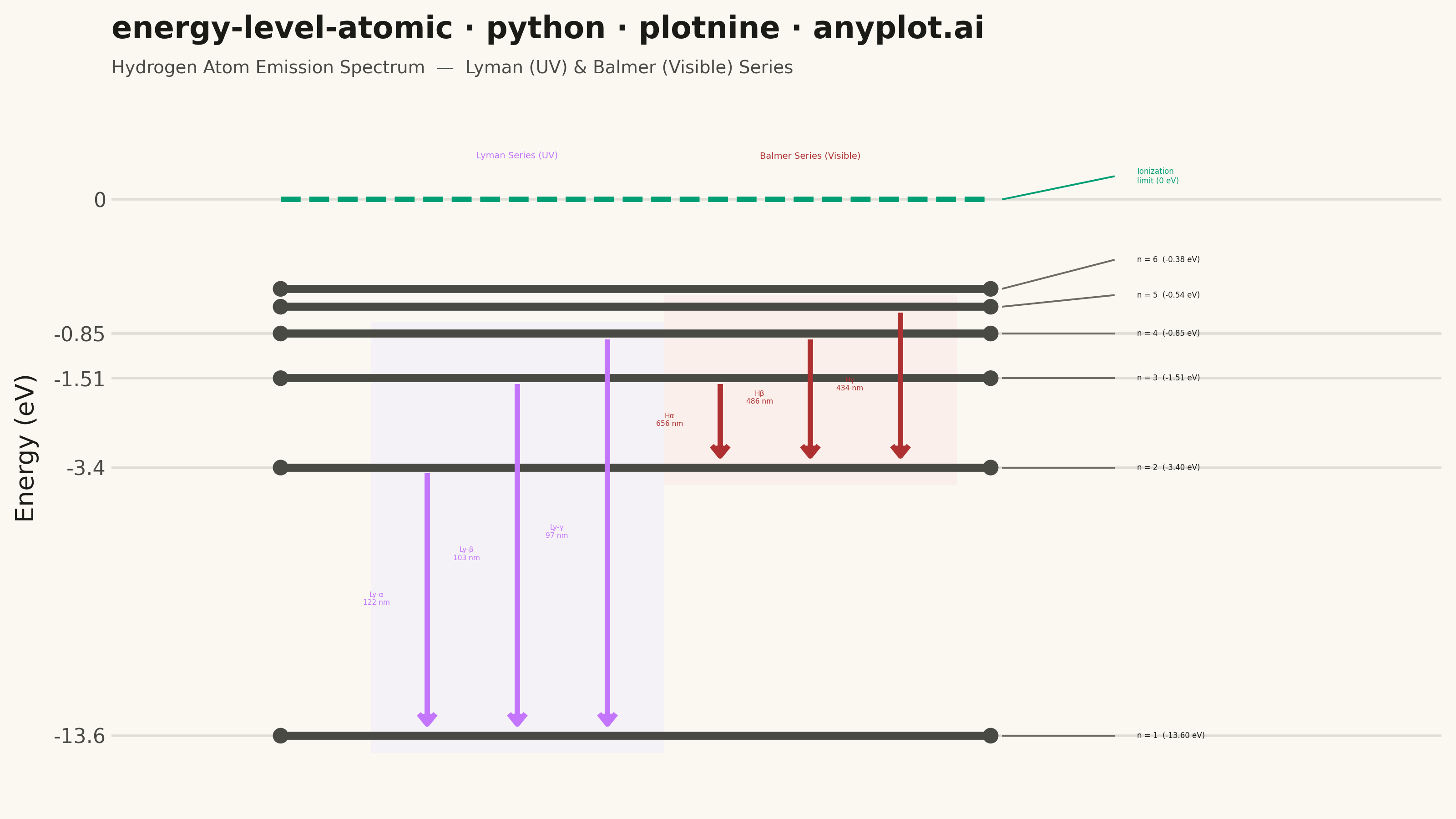
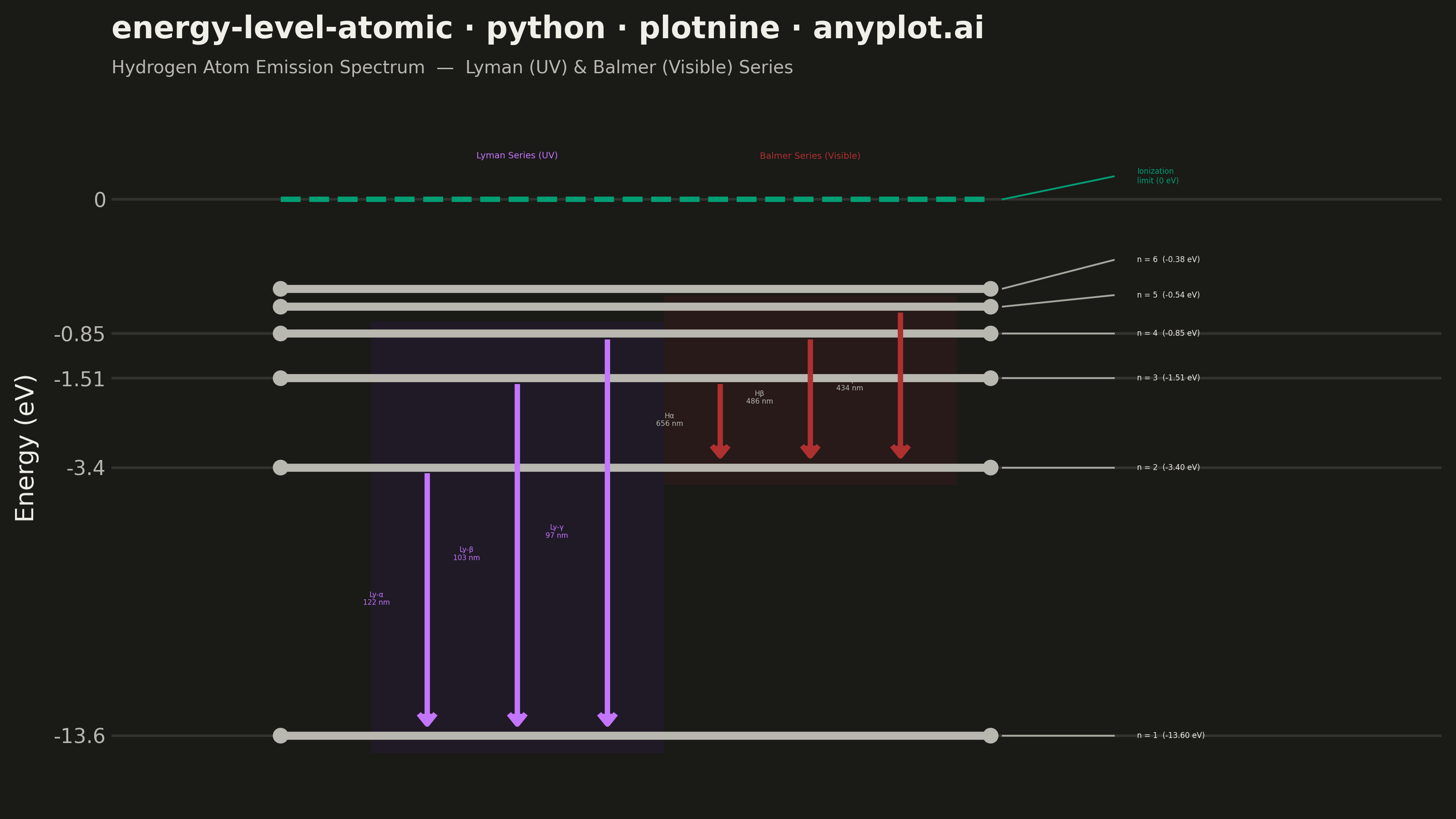
An energy level diagram displays quantized energy states as horizontal lines positioned at their respective energy values, with vertical arrows representing transitions between levels. This visualization reveals the discrete nature of atomic and molecular energy structures, making it essential for understanding spectral series, electron configurations, and quantum state transitions. It provides an intuitive way to connect abstract quantum numbers to observable spectral phenomena.
""" anyplot.ai
energy-level-atomic: Atomic Energy Level Diagram
Library: plotnine 0.15.4 | Python 3.13.13
Quality: 87/100 | Updated: 2026-05-30
"""

import os

import numpy as np
import pandas as pd
from plotnine import (
    aes,
    annotate,
    arrow,
    coord_cartesian,
    element_blank,
    element_line,
    element_rect,
    element_text,
    geom_point,
    geom_rect,
    geom_segment,
    geom_text,
    ggplot,
    labs,
    scale_color_manual,
    scale_fill_identity,
    scale_x_continuous,
    scale_y_continuous,
    theme,
    theme_minimal,
)


# Theme tokens (Imprint palette — see prompts/default-style-guide.md)
THEME = os.getenv("ANYPLOT_THEME", "light")
PAGE_BG = "#FAF8F1" if THEME == "light" else "#1A1A17"
INK = "#1A1A17" if THEME == "light" else "#F0EFE8"
INK_SOFT = "#4A4A44" if THEME == "light" else "#B8B7B0"
INK_MUTED = "#6B6A63" if THEME == "light" else "#A8A79F"

# Imprint palette — semantic spectral mapping (UV=lavender, visible=matte red)
LYMAN_COLOR = "#C475FD"  # Imprint position 2 — lavender → UV spectral region
BALMER_COLOR = "#AE3030"  # Imprint position 5 — matte red → visible light anchor
IONIZATION_COLOR = "#009E73"  # Imprint position 1 — brand green for ionization limit
SERIES_COLORS = {"Lyman (UV)": LYMAN_COLOR, "Balmer (Visible)": BALMER_COLOR}
# Dark theme: Balmer labels over dark brownish-red band have ~2.7:1 contrast; use INK_SOFT instead
BALMER_LABEL_COLOR = BALMER_COLOR if THEME == "light" else INK_SOFT

# Data — Hydrogen atom energy levels (En = -13.6/n² eV)
n_values = np.arange(1, 7)
energies = -13.6 / n_values**2

# Nonlinear visual transform: sign(E)*sqrt(|E|) spreads crowded upper levels
# and compresses the large n=1→n=2 gap (spec: "consider nonlinear scale")
vis_e = np.sign(energies) * np.sqrt(np.abs(energies))

# Energy level lines (partial-width per spec)
levels = pd.DataFrame({"y": vis_e, "x_start": 0.15, "x_end": 0.78})

# Endpoint dots at each end of level lines
endpoints = pd.DataFrame({"x": [0.15] * 6 + [0.78] * 6, "y": list(vis_e) * 2})

# Right-side labels — slight vertical nudge for n=5,6 to prevent overlap
label_y = list(vis_e[:4]) + [vis_e[4] + 0.08, vis_e[5] + 0.20]
labels_df = pd.DataFrame(
    {"y": label_y, "label": [f"n = {n}  ({e:.2f} eV)" for n, e in zip(n_values, energies, strict=True)], "x": 0.91}
)

# Thin connector lines from level endpoints to spread labels
connectors = pd.DataFrame({"x1": [0.79] * 6, "x2": [0.89] * 6, "y1": list(vis_e), "y2": label_y})

# Ionization limit at 0 eV
ion_y = 0.0
ion_label_y = 0.16

# Transitions — grouped by Lyman (UV) and Balmer (Visible) series
energy_lookup = dict(zip(n_values, vis_e, strict=True))
transitions = pd.DataFrame(
    {
        "from_n": [2, 3, 4, 3, 4, 5],
        "to_n": [1, 1, 1, 2, 2, 2],
        "x_pos": [0.28, 0.36, 0.44, 0.54, 0.62, 0.70],
        "series": ["Lyman (UV)"] * 3 + ["Balmer (Visible)"] * 3,
        "label": ["Ly-α\n122 nm", "Ly-β\n103 nm", "Ly-γ\n97 nm", "Hα\n656 nm", "Hβ\n486 nm", "Hγ\n434 nm"],
    }
)
transitions["y_start"] = transitions["from_n"].map(energy_lookup) - 0.04
transitions["y_end"] = transitions["to_n"].map(energy_lookup) + 0.08
transitions["label_y"] = (transitions["y_start"] + transitions["y_end"]) / 2

# Series group labels above the diagram (serve as inline legend)
series_labels = pd.DataFrame(
    {
        "x": [0.36, 0.62],
        "y": [0.30, 0.30],
        "label": ["Lyman Series (UV)", "Balmer Series (Visible)"],
        "series": ["Lyman (UV)", "Balmer (Visible)"],
    }
)

# Shaded bands behind each series (theme-adaptive fill)
band_fill_lyman = "#EDE9FE" if THEME == "light" else "#2A1A40"
band_fill_balmer = "#FEE2E2" if THEME == "light" else "#3C1A1A"
series_bands = pd.DataFrame(
    {
        "xmin": [0.23, 0.49],
        "xmax": [0.49, 0.75],
        "ymin": [vis_e[0] - 0.12, vis_e[1] - 0.12],
        "ymax": [vis_e[3] + 0.08, vis_e[4] + 0.08],
        "fill": [band_fill_lyman, band_fill_balmer],
    }
)

# Y-axis: real eV values at transformed tick positions
y_breaks = [vis_e[0], vis_e[1], vis_e[2], vis_e[3], 0.0]
y_labels = ["-13.6", "-3.4", "-1.51", "-0.85", "0"]

# Title (51 chars — under 67 baseline, default 12pt applies)
title = "energy-level-atomic · python · plotnine · anyplot.ai"

# Build plot — layered grammar: bands → levels → ionization → connectors → labels → arrows
plot = (
    ggplot()
    # Background shaded bands for series grouping
    + geom_rect(
        data=series_bands, mapping=aes(xmin="xmin", xmax="xmax", ymin="ymin", ymax="ymax", fill="fill"), alpha=0.40
    )
    + scale_fill_identity()
    # Energy level lines (structural — INK_SOFT, partial width per spec)
    + geom_segment(data=levels, mapping=aes(x="x_start", xend="x_end", y="y", yend="y"), color=INK_SOFT, size=1.8)
    # Endpoint dots for level lines
    + geom_point(data=endpoints, mapping=aes(x="x", y="y"), color=INK_SOFT, size=2.5)
    # Ionization limit (dashed reference line + label) — brand green structural marker
    + annotate("segment", x=0.15, xend=0.78, y=ion_y, yend=ion_y, color=IONIZATION_COLOR, size=1.2, linetype="dashed")
    + annotate(
        "text", x=0.91, y=ion_label_y, label="Ionization\nlimit (0 eV)", size=3, ha="left", color=IONIZATION_COLOR
    )
    # Connector lines from level endpoints to spread labels
    + geom_segment(data=connectors, mapping=aes(x="x1", xend="x2", y="y1", yend="y2"), color=INK_MUTED, size=0.4)
    # Ionization connector
    + annotate("segment", x=0.79, xend=0.89, y=ion_y, yend=ion_label_y, color=IONIZATION_COLOR, size=0.4)
    # Level labels (right side, primary ink)
    + geom_text(data=labels_df, mapping=aes(x="x", y="y", label="label"), size=3, ha="left", color=INK)
    # Transition arrows (emission = downward, colored by series via scale_color_manual)
    + geom_segment(
        data=transitions,
        mapping=aes(x="x_pos", xend="x_pos", y="y_start", yend="y_end", color="series"),
        size=1.2,
        arrow=arrow(length=0.08, type="closed"),
    )
    # Transition wavelength labels — split by series for theme-adaptive Balmer contrast
    + geom_text(
        data=transitions[transitions["series"] == "Lyman (UV)"],
        mapping=aes(x="x_pos", y="label_y", label="label"),
        size=2.8,
        nudge_x=-0.045,
        color=LYMAN_COLOR,
    )
    + geom_text(
        data=transitions[transitions["series"] == "Balmer (Visible)"],
        mapping=aes(x="x_pos", y="label_y", label="label"),
        size=2.8,
        nudge_x=-0.045,
        color=BALMER_LABEL_COLOR,
    )
    # Series group labels at the top (inline legend, series-matched color)
    + geom_text(data=series_labels, mapping=aes(x="x", y="y", label="label", color="series"), size=3.5)
    # Named color scale — idiomatic plotnine: data-driven aesthetic mapping
    + scale_color_manual(values=SERIES_COLORS)
    + scale_x_continuous(limits=(0.0, 1.18), expand=(0, 0))
    + scale_y_continuous(name="Energy (eV)", breaks=y_breaks, labels=y_labels)
    + coord_cartesian(ylim=(vis_e[0] - 0.25, 0.52))
    + labs(title=title, subtitle="Hydrogen Atom Emission Spectrum  —  Lyman (UV) & Balmer (Visible) Series", x="")
    + theme_minimal()
    + theme(
        figure_size=(8, 4.5),
        plot_title=element_text(size=12, weight="bold", color=INK),
        plot_subtitle=element_text(size=7, color=INK_SOFT),
        axis_title_y=element_text(size=10, color=INK),
        axis_title_x=element_blank(),
        axis_text_y=element_text(size=8, color=INK_SOFT),
        axis_text_x=element_blank(),
        axis_ticks_major_x=element_blank(),
        panel_grid_major_x=element_blank(),
        panel_grid_minor_x=element_blank(),
        panel_grid_minor_y=element_blank(),
        panel_grid_major_y=element_line(alpha=0.12, color=INK),
        plot_background=element_rect(fill=PAGE_BG, color=PAGE_BG),
        panel_background=element_rect(fill=PAGE_BG),
        legend_position="none",
    )
)

# Save
plot.save(f"plot-{THEME}.png", dpi=400, width=8, height=4.5, units="in")
Runnable source as JSON, for any HTTP client: https://api.anyplot.ai/specs/energy-level-atomic/plotnine/code. Any spec id and library id listed in llms-full.txt fit the same URL shape; every URL below is complete and callable.
{
  "spec_id": "energy-level-atomic",
  "language": "python",
  "library": "plotnine",
  "page": "https://anyplot.ai/energy-level-atomic/python/plotnine",
  "hub": "https://anyplot.ai/energy-level-atomic",
  "code_json": "https://api.anyplot.ai/specs/energy-level-atomic/plotnine/code",
  "spec_json": "https://api.anyplot.ai/specs/energy-level-atomic",
  "render_light_png": "https://storage.googleapis.com/anyplot-images/plots/energy-level-atomic/python/plotnine/plot-light.png",
  "render_dark_png": "https://storage.googleapis.com/anyplot-images/plots/energy-level-atomic/python/plotnine/plot-dark.png",
  "quality_score": 87.0,
  "license": "MIT",
  "guide": "https://anyplot.ai/llms.txt"
}
Part of Atomic Energy Level Diagram on anyplot.ai.