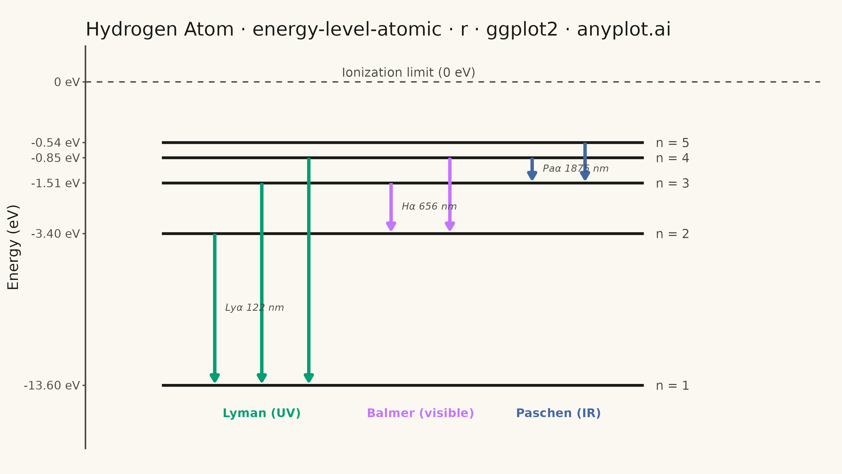
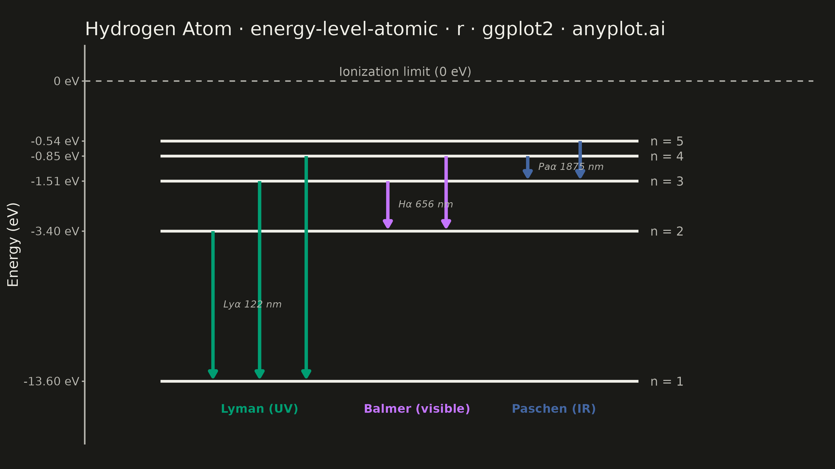
The same plot in 14 other libraries — Python: Altair, Bokeh, lets-plot, Matplotlib, Plotly, plotnine, Pygal, Seaborn; Julia: Makie.jl; JavaScript: Chart.js, D3.js, Apache ECharts, Highcharts, MUI X Charts. Compare all 15 side by side: Atomic Energy Level Diagram in Python, R, Julia and JavaScript.
An energy level diagram displays quantized energy states as horizontal lines positioned at their respective energy values, with vertical arrows representing transitions between levels. This visualization reveals the discrete nature of atomic and molecular energy structures, making it essential for understanding spectral series, electron configurations, and quantum state transitions. It provides an intuitive way to connect abstract quantum numbers to observable spectral phenomena.
#' anyplot.ai
#' energy-level-atomic: Atomic Energy Level Diagram
#' Library: ggplot2 3.5.1 | R 4.4.1
#' Quality: 88/100 | Created: 2026-05-30

library(ggplot2)
library(ragg)

# Theme tokens
THEME       <- Sys.getenv("ANYPLOT_THEME", "light")
PAGE_BG     <- if (THEME == "light") "#FAF8F1" else "#1A1A17"
INK         <- if (THEME == "light") "#1A1A17" else "#F0EFE8"
INK_SOFT    <- if (THEME == "light") "#4A4A44" else "#B8B7B0"
IMPRINT_PALETTE <- c("#009E73", "#C475FD", "#4467A3", "#BD8233",
                     "#AE3030", "#2ABCCD", "#954477", "#99B314")

# Hydrogen atom energy levels (E_n = -13.6 / n^2 eV, n = 1..5)
# Display y = -1/n: spaces levels proportionally to quantum number
# so the crowded upper levels stay legible. Y-axis labels show actual energies.
n_vals  <- 1:5
e_n     <- -13.6 / n_vals^2
y_disp  <- -1.0 / n_vals

levels_df <- data.frame(
  n     = n_vals,
  energy = e_n,
  y     = y_disp,
  label = paste0("n = ", n_vals)
)

# Emission transitions (downward arrows): y_start at upper level, y_end near lower level
# Arrow stops 0.015 display-units above the lower level line so the head clears the line
transitions_df <- data.frame(
  n_upper  = c(2, 3, 4,    3, 4,    4, 5),
  n_lower  = c(1, 1, 1,    2, 2,    3, 3),
  series   = c(
    "Lyman (UV)", "Lyman (UV)", "Lyman (UV)",
    "Balmer (visible)", "Balmer (visible)",
    "Paschen (IR)", "Paschen (IR)"
  ),
  x_pos    = c(0.17, 0.25, 0.33,   0.47, 0.57,   0.71, 0.80),
  wl_label = c("Lyα 122 nm", "", "", "Hα 656 nm", "", "Paα 1875 nm", ""),
  stringsAsFactors = FALSE
)
transitions_df$y_start <- -1.0 / transitions_df$n_upper
transitions_df$y_end   <- -1.0 / transitions_df$n_lower + 0.015
transitions_df$y_mid   <- (transitions_df$y_start + transitions_df$y_end) / 2

series_colors <- c(
  "Lyman (UV)"       = IMPRINT_PALETTE[1],
  "Balmer (visible)" = IMPRINT_PALETTE[2],
  "Paschen (IR)"     = IMPRINT_PALETTE[3]
)

# Subset for wavelength annotations (only labeled transitions)
wl_df <- transitions_df[transitions_df$wl_label != "", ]

# Adaptive title size
title_str  <- "Hydrogen Atom · energy-level-atomic · r · ggplot2 · anyplot.ai"
title_size <- max(8, round(12 * 67 / nchar(title_str)))

# Y-axis breaks at the display positions, labeled with actual energies
y_breaks <- c(y_disp, 0)
y_labels <- c(sprintf("%.2f eV", e_n), "0 eV")

# Plot
p <- ggplot() +
  # Ionization limit
  geom_hline(yintercept = 0, color = INK_SOFT,
             linetype = "dashed", linewidth = 0.45) +
  # Energy level horizontal lines
  geom_segment(
    data = levels_df,
    aes(x = 0.08, xend = 0.90, y = y, yend = y),
    color = INK, linewidth = 0.9
  ) +
  # Quantum number labels (right side)
  geom_text(
    data = levels_df,
    aes(x = 0.92, y = y, label = label),
    hjust = 0, color = INK_SOFT, size = 3.0
  ) +
  # Emission transition arrows
  geom_segment(
    data = transitions_df,
    aes(x = x_pos, xend = x_pos,
        y = y_start, yend = y_end,
        color = series),
    arrow       = arrow(length = unit(0.065, "inches"), type = "closed"),
    linewidth   = 1.1,
    show.legend = FALSE
  ) +
  # Wavelength annotations for representative transitions in each series
  geom_text(
    data = wl_df,
    aes(x = x_pos + 0.018, y = y_mid, label = wl_label),
    color = INK_SOFT, size = 2.4, hjust = 0, fontface = "italic"
  ) +
  # Series labels below the n=1 level
  annotate("text", x = 0.25, y = -1.09, label = "Lyman (UV)",
           color = IMPRINT_PALETTE[1], size = 2.9, fontface = "bold") +
  annotate("text", x = 0.52, y = -1.09, label = "Balmer (visible)",
           color = IMPRINT_PALETTE[2], size = 2.9, fontface = "bold") +
  annotate("text", x = 0.755, y = -1.09, label = "Paschen (IR)",
           color = IMPRINT_PALETTE[3], size = 2.9, fontface = "bold") +
  # Ionization label (size increased to 3.0 for better mobile readability)
  annotate("text", x = 0.50, y = 0.032, label = "Ionization limit (0 eV)",
           color = INK_SOFT, size = 3.0, hjust = 0.5) +
  scale_color_manual(values = series_colors) +
  scale_x_continuous(limits = c(-0.05, 1.20), expand = c(0, 0)) +
  scale_y_continuous(
    name   = "Energy (eV)",
    breaks = y_breaks,
    labels = y_labels,
    limits = c(-1.15, 0.06)
  ) +
  coord_cartesian(clip = "off") +
  labs(title = title_str, x = NULL) +
  theme_minimal(base_size = 8) +
  theme(
    plot.background  = element_rect(fill = PAGE_BG, color = PAGE_BG),
    panel.background = element_rect(fill = PAGE_BG, color = NA),
    panel.grid.major = element_blank(),
    panel.grid.minor = element_blank(),
    panel.border     = element_blank(),
    axis.title.y     = element_text(color = INK,      size = 10),
    axis.title.x     = element_blank(),
    axis.text.y      = element_text(color = INK_SOFT, size = 8),
    axis.text.x      = element_blank(),
    axis.ticks.x     = element_blank(),
    axis.ticks.y     = element_line(color = INK_SOFT, linewidth = 0.4),
    axis.line.y      = element_line(color = INK_SOFT, linewidth = 0.5),
    plot.title       = element_text(color = INK, size = title_size, face = "plain"),
    legend.position  = "none",
    plot.margin      = margin(15, 15, 15, 5)
  )

# Save
ggsave(
  filename = sprintf("plot-%s.png", THEME),
  plot     = p,
  device   = ragg::agg_png,
  width    = 8,
  height   = 4.5,
  units    = "in",
  dpi      = 400
)
Runnable source as JSON, for any HTTP client: https://api.anyplot.ai/specs/energy-level-atomic/ggplot2/code. Any spec id and library id listed in llms-full.txt fit the same URL shape; every URL below is complete and callable.
{
  "spec_id": "energy-level-atomic",
  "language": "r",
  "library": "ggplot2",
  "page": "https://anyplot.ai/energy-level-atomic/r/ggplot2",
  "hub": "https://anyplot.ai/energy-level-atomic",
  "code_json": "https://api.anyplot.ai/specs/energy-level-atomic/ggplot2/code",
  "spec_json": "https://api.anyplot.ai/specs/energy-level-atomic",
  "render_light_png": "https://storage.googleapis.com/anyplot-images/plots/energy-level-atomic/r/ggplot2/plot-light.png",
  "render_dark_png": "https://storage.googleapis.com/anyplot-images/plots/energy-level-atomic/r/ggplot2/plot-dark.png",
  "quality_score": 88.0,
  "license": "MIT",
  "guide": "https://anyplot.ai/llms.txt"
}
Part of Atomic Energy Level Diagram on anyplot.ai.