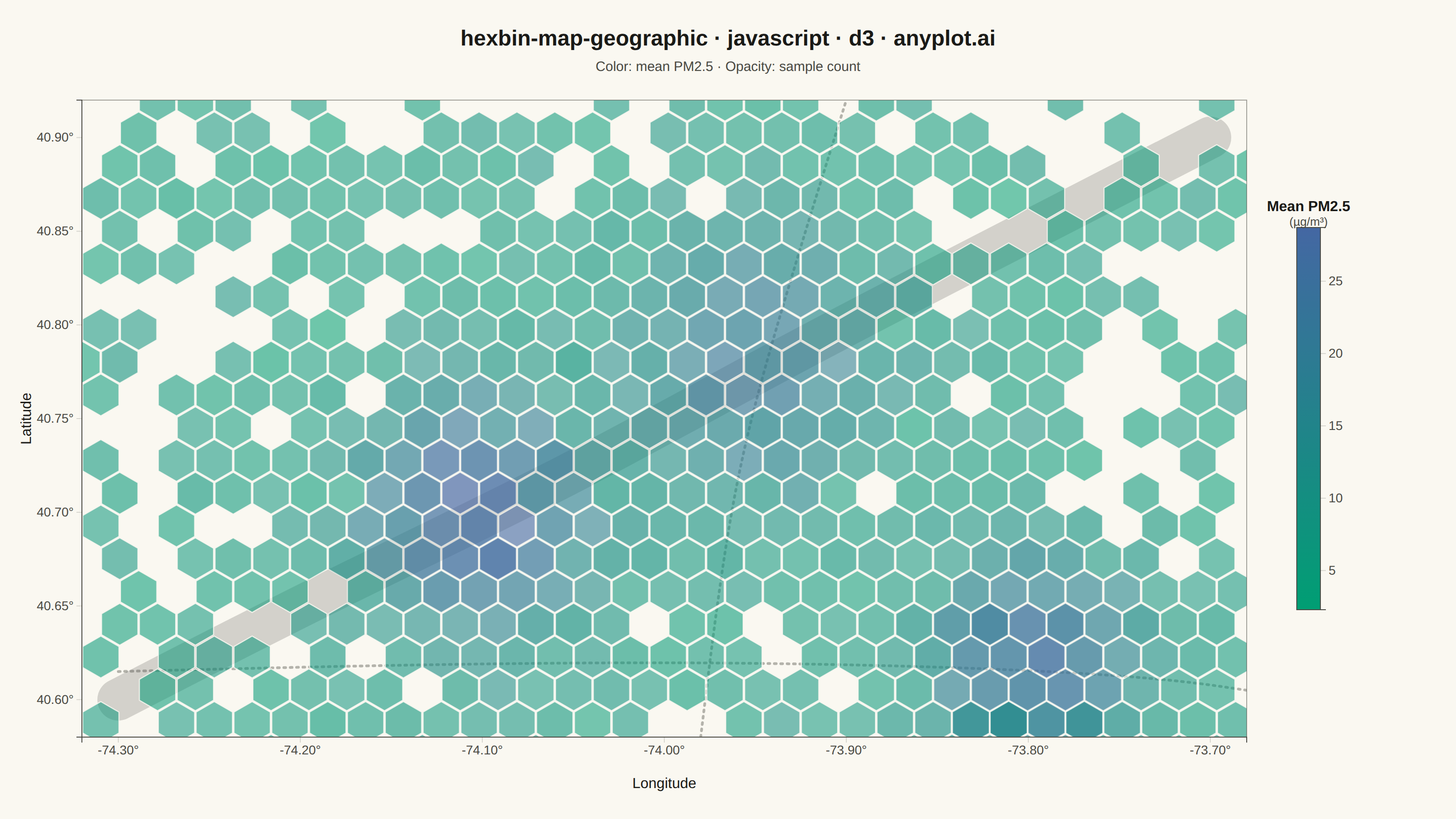
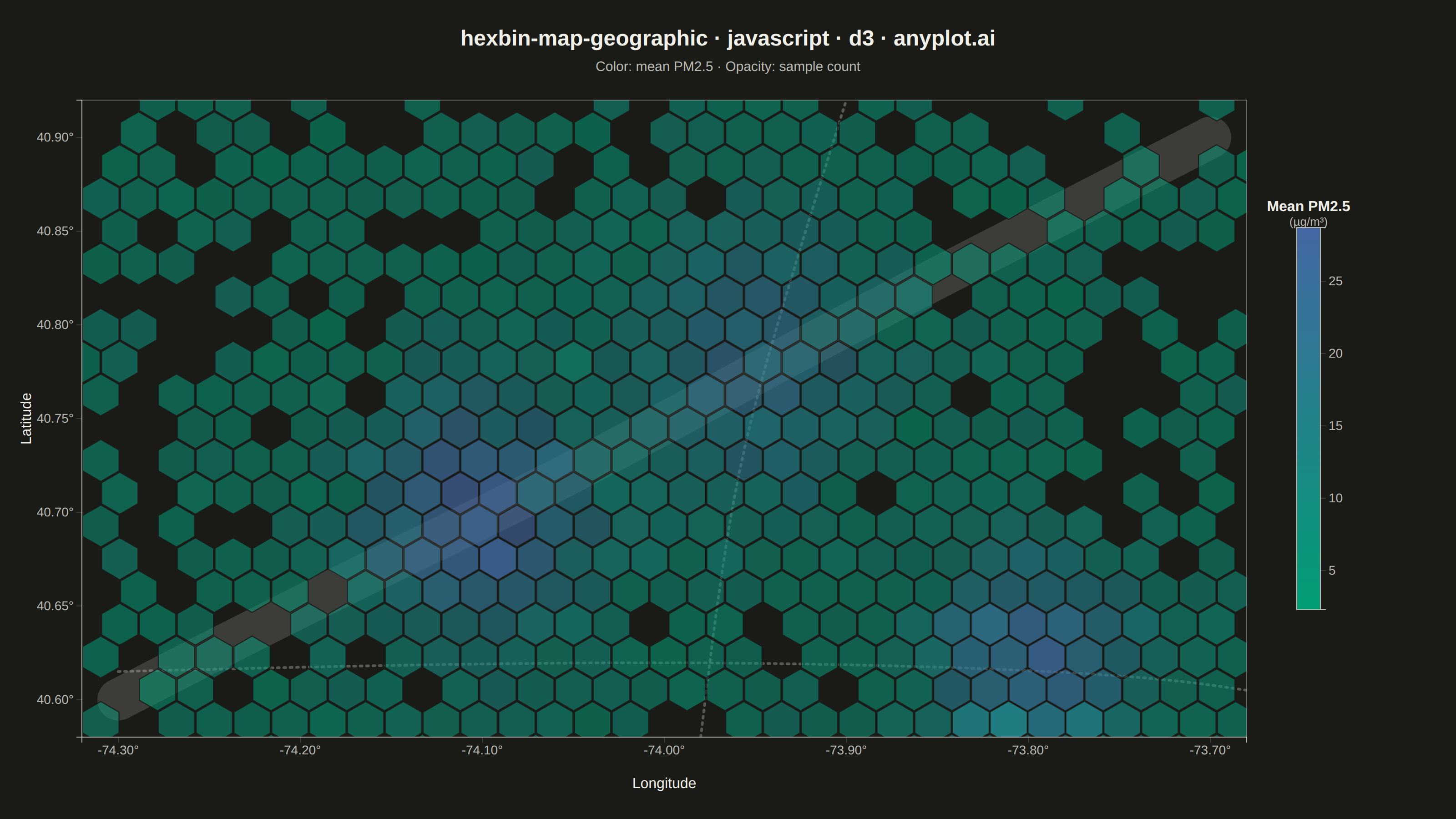
The same plot in 14 other libraries — JavaScript: Chart.js, Apache ECharts, Highcharts, MUI X Charts; Python: Altair, Bokeh, lets-plot, Matplotlib, Plotly, plotnine, Pygal, Seaborn; R: ggplot2; Julia: Makie.jl. Compare all 15 side by side: Hexagonal Binning Map in Python, R, Julia and JavaScript.
A geographic map visualization that aggregates point data into hexagonal cells, displaying density or aggregated values per cell using color intensity. Unlike continuous heatmaps that use kernel density estimation, hexbin maps provide discrete binning that clearly shows data aggregation boundaries. The hexagonal grid is superior to square grids due to isotropy (equal distance to neighboring cells) and better visual continuity, making it ideal for spatial statistics and urban data analysis.
// anyplot.ai
// hexbin-map-geographic: Hexagonal Binning Map
// Library: d3 7.9.0 | JavaScript 22.23.2
// Quality: 92/100 | Created: 2026-08-25

const t = window.ANYPLOT_TOKENS;
const { width, height } = window.ANYPLOT_SIZE;

// --- Deterministic PRNG (LCG + Box-Muller) ----------------------------------
let seed = 42;
function nextRandom() {
  seed = (1103515245 * seed + 12345) % 2147483648;
  return seed / 2147483648;
}
function randomGaussian() {
  const u1 = Math.max(nextRandom(), 1e-6);
  const u2 = nextRandom();
  return Math.sqrt(-2 * Math.log(u1)) * Math.cos(2 * Math.PI * u2);
}
function clamp(value, lo, hi) {
  return Math.max(lo, Math.min(hi, value));
}

// --- Data: air-quality sensor readings across a river-adjacent metro area --
const lonMin = -74.32;
const lonMax = -73.68;
const latMin = 40.58;
const latMax = 40.92;

const hotspots = [
  { lon: -74.1, lat: 40.7, spread: 0.045, boost: 24 }, // industrial zone
  { lon: -73.95, lat: 40.78, spread: 0.05, boost: 16 }, // highway interchange
  { lon: -73.8, lat: 40.62, spread: 0.04, boost: 20 }, // downtown core
];

const nPoints = 5000;
const points = [];
for (let i = 0; i < nPoints; i += 1) {
  const roll = nextRandom();
  let lon;
  let lat;
  let baseValue;
  if (roll < 0.72) {
    const hs = hotspots[Math.min(hotspots.length - 1, Math.floor(nextRandom() * hotspots.length))];
    lon = hs.lon + randomGaussian() * hs.spread;
    lat = hs.lat + randomGaussian() * hs.spread;
    const dist = Math.hypot(lon - hs.lon, lat - hs.lat) / hs.spread;
    baseValue = 7 + hs.boost * Math.exp(-0.5 * dist * dist) + randomGaussian() * 2;
  } else {
    lon = lonMin + nextRandom() * (lonMax - lonMin);
    lat = latMin + nextRandom() * (latMax - latMin);
    baseValue = 6 + randomGaussian() * 1.5;
  }
  points.push({
    lon: clamp(lon, lonMin, lonMax),
    lat: clamp(lat, latMin, latMax),
    value: Math.max(1, baseValue),
  });
}

// River waypoints, used only as base-map context under the hexagons
const riverLonLat = [
  [-74.3, 40.6],
  [-74.18, 40.66],
  [-74.05, 40.72],
  [-73.94, 40.78],
  [-73.82, 40.84],
  [-73.7, 40.9],
];

// Street waypoints — a second base-map context cue alongside the river, thin
// and neutral so they read as street lines rather than data
const streetLonLats = [
  [
    [-74.3, 40.615],
    [-74.0, 40.622],
    [-73.75, 40.615],
    [-73.68, 40.605],
  ],
  [
    [-73.98, 40.58],
    [-73.965, 40.7],
    [-73.945, 40.78],
    [-73.9, 40.92],
  ],
];

// --- Layout -------------------------------------------------------------
const margin = { top: 110, right: 230, bottom: 90, left: 90 };
const mapW = width - margin.left - margin.right;
const mapH = height - margin.top - margin.bottom;

const xScale = d3.scaleLinear().domain([lonMin, lonMax]).range([0, mapW]);
const yScale = d3.scaleLinear().domain([latMin, latMax]).range([mapH, 0]);

// --- Hexagonal binning (axial cube-rounding, pointy-top hexagons) ----------
const hexSize = 24; // center-to-corner, CSS px

function cubeRound(qf, rf) {
  const xf = qf;
  const zf = rf;
  const yf = -xf - zf;
  let rx = Math.round(xf);
  let ry = Math.round(yf);
  let rz = Math.round(zf);
  const dx = Math.abs(rx - xf);
  const dy = Math.abs(ry - yf);
  const dz = Math.abs(rz - zf);
  if (dx > dy && dx > dz) rx = -ry - rz;
  else if (dy > dz) ry = -rx - rz;
  else rz = -rx - ry;
  return [rx, rz];
}

function pixelToAxial(px, py, size) {
  const q = ((Math.sqrt(3) / 3) * px - py / 3) / size;
  const r = ((2 / 3) * py) / size;
  return cubeRound(q, r);
}

function axialToPixel(q, r, size) {
  return [size * (Math.sqrt(3) * q + (Math.sqrt(3) / 2) * r), size * 1.5 * r];
}

function hexPoints(cx, cy, size) {
  return d3.range(6).map((i) => {
    const angle = (Math.PI / 180) * (60 * i - 30);
    return [cx + size * Math.cos(angle), cy + size * Math.sin(angle)];
  });
}

const bins = new Map();
for (const p of points) {
  const px = xScale(p.lon);
  const py = yScale(p.lat);
  const [q, r] = pixelToAxial(px, py, hexSize);
  const key = `${q},${r}`;
  let bin = bins.get(key);
  if (!bin) {
    bin = { q, r, count: 0, sum: 0 };
    bins.set(key, bin);
  }
  bin.count += 1;
  bin.sum += p.value;
}
const hexData = Array.from(bins.values()).map((b) => {
  const center = axialToPixel(b.q, b.r, hexSize);
  return { ...b, mean: b.sum / b.count, center };
});

const meanExtent = d3.extent(hexData, (d) => d.mean);
const countMax = d3.max(hexData, (d) => d.count);
const color = d3.scaleSequential(d3.interpolateRgbBasis(t.seq)).domain(meanExtent);
const hexOpacity = d3.scaleLinear().domain([1, countMax]).range([0.55, 0.92]).clamp(true);
// Sparse cells get a firmer stroke to stay legible against the page background;
// dense, high-fill-opacity cells get a near-invisible stroke so the frame
// doesn't compete with the color/opacity encoding.
const hexStrokeOpacity = d3.scaleLinear().domain([1, countMax]).range([0.85, 0.18]).clamp(true);

// --- SVG mount ---------------------------------------------------------
const svg = d3.select("#container").append("svg").attr("width", width).attr("height", height);
const g = svg.append("g").attr("transform", `translate(${margin.left},${margin.top})`);

svg
  .append("defs")
  .append("clipPath")
  .attr("id", "map-clip")
  .append("rect")
  .attr("width", mapW)
  .attr("height", mapH);
const mapG = g.append("g").attr("clip-path", "url(#map-clip)");

// River — geographic base-map context, drawn under the hexagons
const riverLine = d3
  .line()
  .x((d) => xScale(d[0]))
  .y((d) => yScale(d[1]))
  .curve(d3.curveBasis);
mapG
  .append("path")
  .datum(riverLonLat)
  .attr("d", riverLine)
  .attr("fill", "none")
  .attr("stroke", t.inkSoft)
  .attr("stroke-width", 46)
  .attr("stroke-linecap", "round")
  .attr("stroke-linejoin", "round")
  .attr("opacity", 0.22);

// Streets — thin neutral lines crossing the hotspots, a second geographic
// context cue so the map reads as more than a coordinate grid with one
// decoration
const streetLine = d3
  .line()
  .x((d) => xScale(d[0]))
  .y((d) => yScale(d[1]))
  .curve(d3.curveBasis);
mapG
  .selectAll("path.street")
  .data(streetLonLats)
  .join("path")
  .attr("class", "street")
  .attr("d", streetLine)
  .attr("fill", "none")
  .attr("stroke", t.inkSoft)
  .attr("stroke-width", 3)
  .attr("stroke-linecap", "round")
  .attr("stroke-dasharray", "2,5")
  .attr("opacity", 0.4);

// Tooltip — real hover, only live in the exported interactive HTML
const tooltip = d3
  .select("#container")
  .append("div")
  .style("position", "fixed")
  .style("pointer-events", "none")
  .style("opacity", 0)
  .style("background", t.elevatedBg)
  .style("color", t.ink)
  .style("border", `1px solid ${t.grid}`)
  .style("border-radius", "6px")
  .style("padding", "8px 10px")
  .style("font-size", "13px")
  .style("font-family", "sans-serif")
  .style("line-height", "1.5")
  .style("box-shadow", "0 2px 8px rgba(0,0,0,0.25)")
  .style("transition", "opacity 0.1s linear");

// Hexagons — mean PM2.5 per cell, with count-driven transparency so the
// river shows through sparsely-sampled bins
mapG
  .selectAll("polygon.hex")
  .data(hexData)
  .join("polygon")
  .attr("class", "hex")
  .attr("points", (d) =>
    hexPoints(d.center[0], d.center[1], hexSize * 0.96)
      .map((p) => p.join(","))
      .join(" "),
  )
  .attr("fill", (d) => color(d.mean))
  .attr("fill-opacity", (d) => hexOpacity(d.count))
  .attr("stroke", t.pageBg)
  .attr("stroke-width", 1.2)
  .attr("stroke-opacity", (d) => hexStrokeOpacity(d.count))
  .style("cursor", "pointer")
  .on("mouseenter", function (event, d) {
    d3.select(this).attr("stroke", t.ink).attr("stroke-width", 2).attr("stroke-opacity", 1);
    tooltip.style("opacity", 1);
  })
  .on("mousemove", function (event, d) {
    const lon = xScale.invert(d.center[0]);
    const lat = yScale.invert(d.center[1]);
    tooltip
      .style("left", `${event.clientX + 16}px`)
      .style("top", `${event.clientY + 16}px`)
      .html(
        `<strong>Count:</strong> ${d.count}<br>` +
          `<strong>Sum:</strong> ${d.sum.toFixed(1)} µg/m³<br>` +
          `<strong>Mean:</strong> ${d.mean.toFixed(1)} µg/m³<br>` +
          `<strong>Center:</strong> ${lon.toFixed(3)}°, ${lat.toFixed(3)}°`,
      );
  })
  .on("mouseleave", function (event, d) {
    d3.select(this)
      .attr("stroke", t.pageBg)
      .attr("stroke-width", 1.2)
      .attr("stroke-opacity", hexStrokeOpacity(d.count));
    tooltip.style("opacity", 0);
  });

// --- Map frame + lon/lat axes -----------------------------------------
g.append("rect")
  .attr("width", mapW)
  .attr("height", mapH)
  .attr("fill", "none")
  .attr("stroke", t.inkSoft)
  .attr("stroke-width", 1)
  .attr("stroke-opacity", 0.5);

const lonAxis = d3
  .axisBottom(xScale)
  .ticks(6)
  .tickFormat((d) => `${d.toFixed(2)}°`);
const latAxis = d3
  .axisLeft(yScale)
  .ticks(5)
  .tickFormat((d) => `${d.toFixed(2)}°`);

const lonAxisG = g.append("g").attr("transform", `translate(0,${mapH})`).call(lonAxis);
const latAxisG = g.append("g").call(latAxis);
for (const axisG of [lonAxisG, latAxisG]) {
  axisG.selectAll("text").attr("fill", t.inkSoft).style("font-size", "14px");
  axisG.selectAll("line").attr("stroke", t.grid);
  axisG.select(".domain").attr("stroke", t.inkSoft);
}

g.append("text")
  .attr("x", mapW / 2)
  .attr("y", mapH + 56)
  .attr("text-anchor", "middle")
  .attr("fill", t.ink)
  .style("font-size", "16px")
  .text("Longitude");

g.append("text")
  .attr("transform", "rotate(-90)")
  .attr("x", -mapH / 2)
  .attr("y", -56)
  .attr("text-anchor", "middle")
  .attr("fill", t.ink)
  .style("font-size", "16px")
  .text("Latitude");

// --- Legend --------------------------------------------------------------
const legendW = 26;
const legendH = mapH * 0.6;
const legendX = mapW + 55;
const legendY = (mapH - legendH) / 2;
const nStops = 10;

svg
  .append("defs")
  .append("linearGradient")
  .attr("id", "legend-gradient")
  .attr("x1", "0%")
  .attr("y1", "100%")
  .attr("x2", "0%")
  .attr("y2", "0%")
  .selectAll("stop")
  .data(d3.range(nStops + 1))
  .join("stop")
  .attr("offset", (d) => `${(d / nStops) * 100}%`)
  .attr("stop-color", (d) => color(meanExtent[0] + (d / nStops) * (meanExtent[1] - meanExtent[0])));

const legendG = g.append("g").attr("transform", `translate(${legendX},${legendY})`);
legendG
  .append("rect")
  .attr("width", legendW)
  .attr("height", legendH)
  .attr("fill", "url(#legend-gradient)")
  .attr("stroke", t.inkSoft)
  .attr("stroke-width", 1);

const legendScale = d3.scaleLinear().domain(meanExtent).range([legendH, 0]);
const legendAxis = d3
  .axisRight(legendScale)
  .ticks(5)
  .tickFormat((d) => d.toFixed(0));
const legendAxisG = legendG.append("g").attr("transform", `translate(${legendW},0)`).call(legendAxis);
legendAxisG.selectAll("text").attr("fill", t.inkSoft).style("font-size", "14px");
legendAxisG.selectAll("line").attr("stroke", t.grid);
legendAxisG.select(".domain").attr("stroke", t.inkSoft);

legendG
  .append("text")
  .attr("x", legendW / 2)
  .attr("y", -18)
  .attr("text-anchor", "middle")
  .attr("fill", t.ink)
  .style("font-size", "16px")
  .style("font-weight", "600")
  .text("Mean PM2.5");
legendG
  .append("text")
  .attr("x", legendW / 2)
  .attr("y", -2)
  .attr("text-anchor", "middle")
  .attr("fill", t.inkSoft)
  .style("font-size", "13px")
  .text("(µg/m³)");

// --- Title -----------------------------------------------------------------
svg
  .append("text")
  .attr("x", width / 2)
  .attr("y", 50)
  .attr("text-anchor", "middle")
  .attr("fill", t.ink)
  .style("font-size", "24px")
  .style("font-weight", "600")
  .text("hexbin-map-geographic · javascript · d3 · anyplot.ai");

svg
  .append("text")
  .attr("x", width / 2)
  .attr("y", 78)
  .attr("text-anchor", "middle")
  .attr("fill", t.inkSoft)
  .style("font-size", "15px")
  .text("Color: mean PM2.5 · Opacity: sample count");
Runnable source as JSON, for any HTTP client: https://api.anyplot.ai/specs/hexbin-map-geographic/d3/code. Any spec id and library id listed in llms-full.txt fit the same URL shape; every URL below is complete and callable.
{
  "spec_id": "hexbin-map-geographic",
  "language": "javascript",
  "library": "d3",
  "page": "https://anyplot.ai/hexbin-map-geographic/javascript/d3",
  "hub": "https://anyplot.ai/hexbin-map-geographic",
  "code_json": "https://api.anyplot.ai/specs/hexbin-map-geographic/d3/code",
  "spec_json": "https://api.anyplot.ai/specs/hexbin-map-geographic",
  "render_light_png": "https://storage.googleapis.com/anyplot-images/plots/hexbin-map-geographic/javascript/d3/plot-light.png",
  "render_dark_png": "https://storage.googleapis.com/anyplot-images/plots/hexbin-map-geographic/javascript/d3/plot-dark.png",
  "interactive_light_html": "https://storage.googleapis.com/anyplot-images/plots/hexbin-map-geographic/javascript/d3/plot-light.html",
  "interactive_dark_html": "https://storage.googleapis.com/anyplot-images/plots/hexbin-map-geographic/javascript/d3/plot-dark.html",
  "quality_score": 92.0,
  "license": "MIT",
  "guide": "https://anyplot.ai/llms.txt"
}
Part of Hexagonal Binning Map on anyplot.ai.