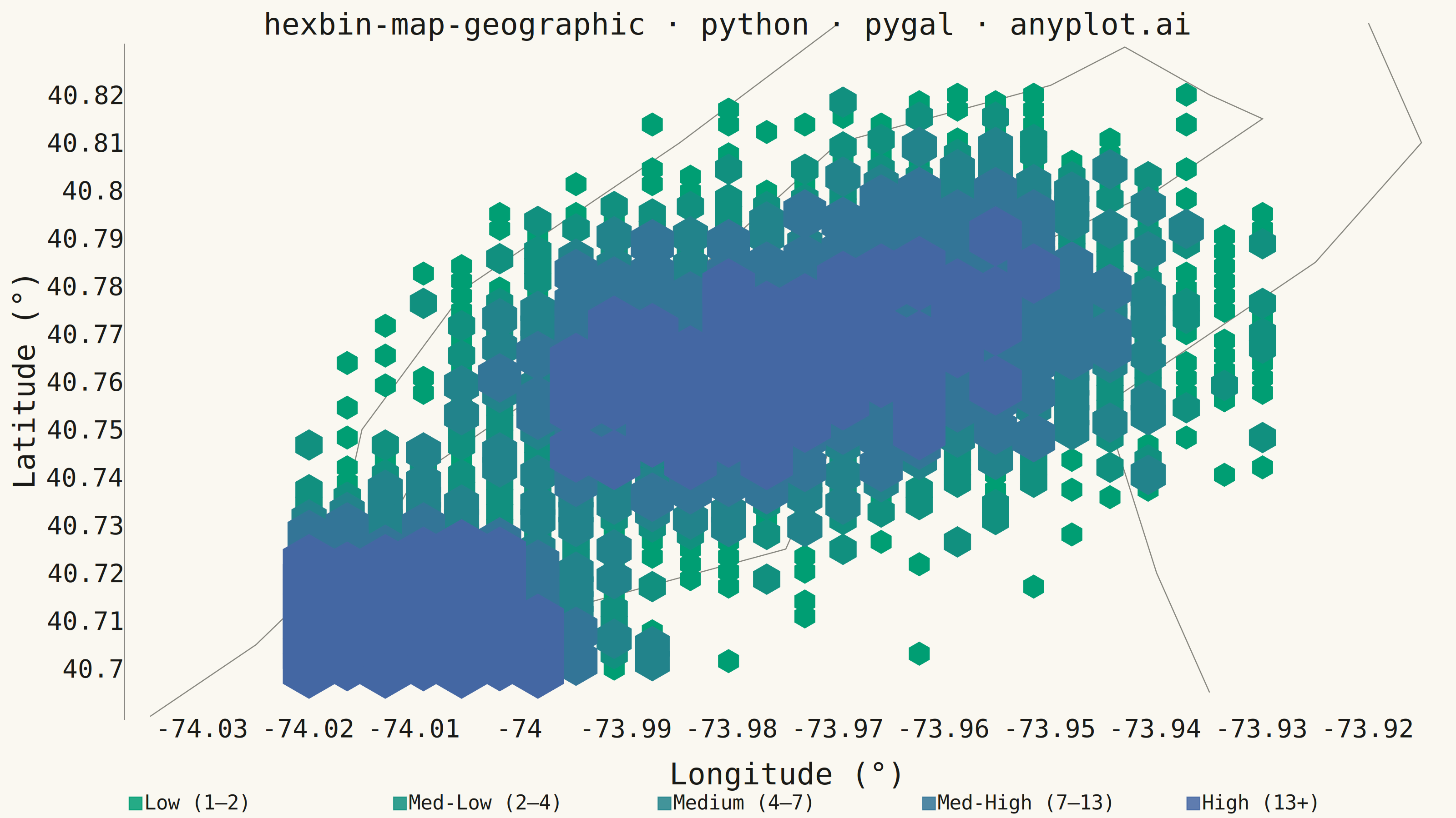
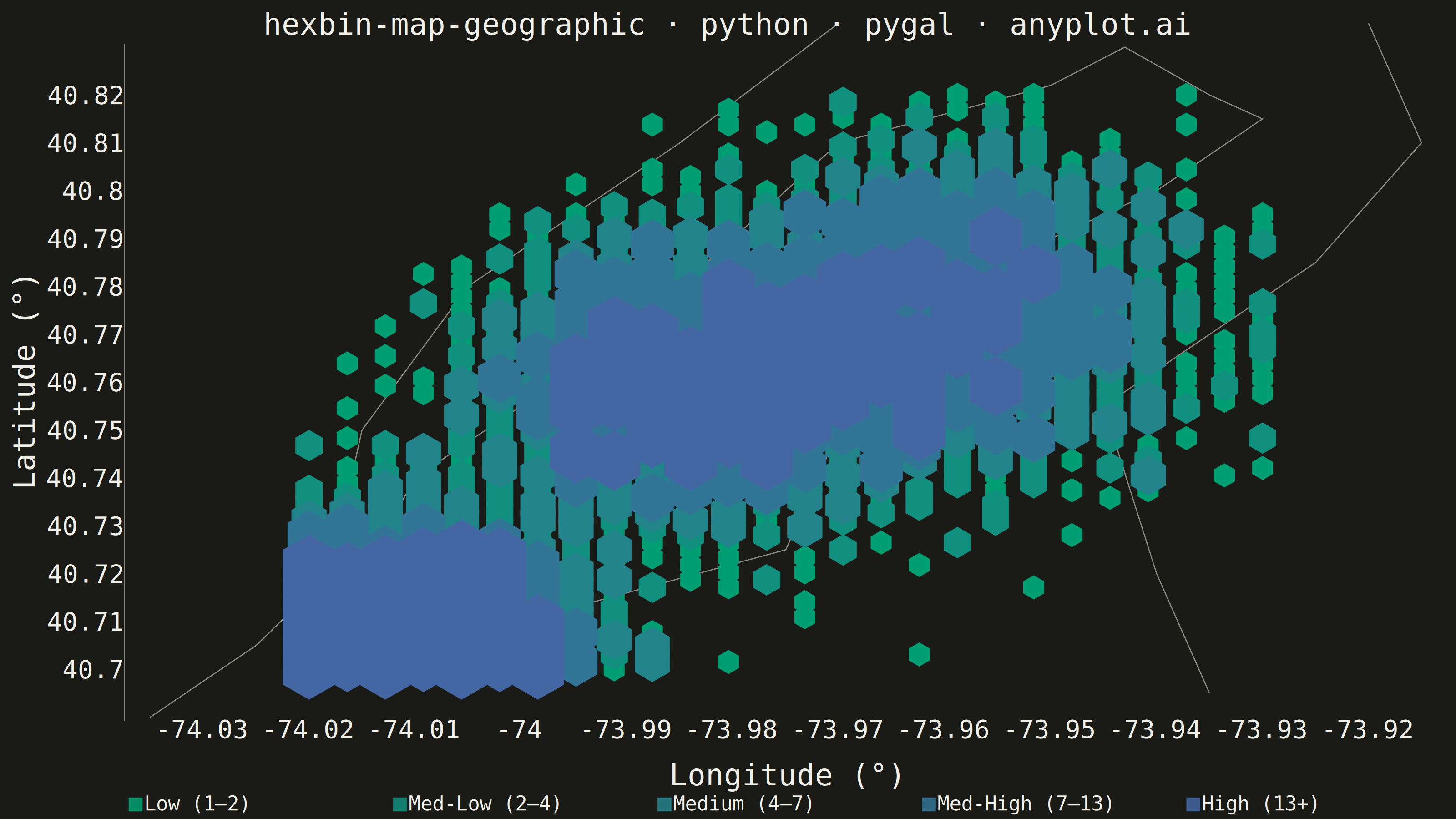
A geographic map visualization that aggregates point data into hexagonal cells, displaying density or aggregated values per cell using color intensity. Unlike continuous heatmaps that use kernel density estimation, hexbin maps provide discrete binning that clearly shows data aggregation boundaries. The hexagonal grid is superior to square grids due to isotropy (equal distance to neighboring cells) and better visual continuity, making it ideal for spatial statistics and urban data analysis.
""" anyplot.ai
hexbin-map-geographic: Hexagonal Binning Map
Library: pygal 3.1.0 | Python 3.13.13
Quality: 84/100 | Updated: 2026-05-27
"""

import math
import os
import re
import sys
from collections import defaultdict


# Fix module name conflict (this file is named pygal.py)
_cwd = sys.path[0] if sys.path and sys.path[0] else None
if _cwd:
    sys.path.remove(_cwd)

import cairosvg
import numpy as np
import pygal
from pygal.style import Style


if _cwd:
    sys.path.insert(0, _cwd)

# Theme tokens
THEME = os.getenv("ANYPLOT_THEME", "light")
PAGE_BG = "#FAF8F1" if THEME == "light" else "#1A1A17"
INK = "#1A1A17" if THEME == "light" else "#F0EFE8"
INK_MUTED = "#6B6A63" if THEME == "light" else "#A8A79F"

# imprint_seq: #009E73 → #4467A3 (5 evenly-spaced stops, low → high density)
seq_stops = ("#009E73", "#11907F", "#22838B", "#337597", "#4467A3")
n_density_bins = 5

# Data — NYC taxi pickup locations (Manhattan)
np.random.seed(42)
n_points = 5000
lat_min, lat_max = 40.70, 40.82
lon_min, lon_max = -74.02, -73.93

c1_lat = np.random.normal(40.758, 0.015, n_points // 3)
c1_lon = np.random.normal(-73.985, 0.01, n_points // 3)
c1_vals = np.random.exponential(25, n_points // 3)

c2_lat = np.random.normal(40.710, 0.012, n_points // 3)
c2_lon = np.random.normal(-74.010, 0.008, n_points // 3)
c2_vals = np.random.exponential(35, n_points // 3)

c3_lat = np.random.normal(40.775, 0.018, n_points // 3)
c3_lon = np.random.normal(-73.960, 0.012, n_points // 3)
c3_vals = np.random.exponential(20, n_points // 3)

lat = np.clip(np.concatenate([c1_lat, c2_lat, c3_lat]), lat_min, lat_max)
lon = np.clip(np.concatenate([c1_lon, c2_lon, c3_lon]), lon_min, lon_max)
values = np.concatenate([c1_vals, c2_vals, c3_vals])

# Hexagonal binning with count and fare aggregation
gridsize = 25
x_arr = np.asarray(lon)
y_arr = np.asarray(lat)
x_min_v, x_max_v = x_arr.min(), x_arr.max()
y_min_v = y_arr.min()
hex_width = (x_max_v - x_min_v) / gridsize
hex_height = hex_width * np.sqrt(3) / 2

bins = defaultdict(lambda: {"count": 0, "sum": 0.0})
for xi, yi, vi in zip(x_arr, y_arr, values, strict=True):
    col = (xi - x_min_v) / hex_width
    row_offset = (int(col) % 2) * 0.5
    row = (yi - y_min_v) / hex_height - row_offset
    col_idx = int(round(col))
    row_idx = int(round(row))
    bins[(col_idx, row_idx)]["count"] += 1
    bins[(col_idx, row_idx)]["sum"] += vi

hex_data = []
for (col_idx, row_idx), data in bins.items():
    cx = x_min_v + col_idx * hex_width
    row_offset = (col_idx % 2) * 0.5
    cy = y_min_v + (row_idx + row_offset) * hex_height
    count = data["count"]
    total = data["sum"]
    mean = total / count if count > 0 else 0
    hex_data.append({"lon": cx, "lat": cy, "count": count, "sum": total, "mean": mean})

counts = np.array([h["count"] for h in hex_data])

# Percentile-based bin edges for balanced distribution
bin_edges = np.percentile(counts, [0, 20, 40, 60, 80, 100])
for i in range(1, len(bin_edges)):
    if bin_edges[i] <= bin_edges[i - 1]:
        bin_edges[i] = bin_edges[i - 1] + 1

# Shortened labels to prevent legend truncation
bin_labels = [
    f"Low ({int(bin_edges[0])}–{int(bin_edges[1])})",
    f"Med-Low ({int(bin_edges[1])}–{int(bin_edges[2])})",
    f"Medium ({int(bin_edges[2])}–{int(bin_edges[3])})",
    f"Med-High ({int(bin_edges[3])}–{int(bin_edges[4])})",
    f"High ({int(bin_edges[4])}+)",
]

# Geographic outlines (Manhattan island + waterways)
manhattan_outline = [
    (-74.020, 40.700),
    (-74.010, 40.705),
    (-74.000, 40.710),
    (-73.975, 40.725),
    (-73.970, 40.750),
    (-73.965, 40.775),
    (-73.940, 40.800),
    (-73.930, 40.815),
    (-73.935, 40.820),
    (-73.943, 40.830),
    (-73.950, 40.822),
    (-73.970, 40.810),
    (-73.990, 40.770),
    (-74.010, 40.740),
    (-74.015, 40.720),
    (-74.020, 40.700),
]
hudson_river = [
    (-74.035, 40.690),
    (-74.025, 40.705),
    (-74.018, 40.720),
    (-74.015, 40.750),
    (-74.005, 40.780),
    (-73.985, 40.810),
    (-73.970, 40.835),
]
east_river = [
    (-73.935, 40.695),
    (-73.940, 40.720),
    (-73.945, 40.755),
    (-73.925, 40.785),
    (-73.915, 40.810),
    (-73.920, 40.835),
]

title = "hexbin-map-geographic · python · pygal · anyplot.ai"

custom_style = Style(
    background=PAGE_BG,
    plot_background=PAGE_BG,
    foreground=INK,
    foreground_strong=INK,
    foreground_subtle=INK_MUTED,
    guide_stroke_color="transparent",
    colors=(INK_MUTED, INK_MUTED, INK_MUTED) + seq_stops,
    opacity=0.85,
    opacity_hover=0.95,
    title_font_size=66,
    label_font_size=56,
    major_label_font_size=44,
    legend_font_size=44,
    value_font_size=36,
    stroke_width=2.5,
)

chart = pygal.XY(
    width=3200,
    height=1800,
    style=custom_style,
    title=title,
    x_title="Longitude (°)",
    y_title="Latitude (°)",
    show_legend=True,
    legend_at_bottom=True,
    legend_at_bottom_columns=5,
    legend_box_size=28,
    stroke=False,
    dots_size=30,
    show_x_guides=False,
    show_y_guides=False,
    explicit_size=True,
    print_values=False,
    xrange=(lon_min - 0.015, lon_max + 0.015),
    range=(lat_min - 0.008, lat_max + 0.008),
)

# Geographic boundaries (excluded from legend via None label)
chart.add(None, manhattan_outline, stroke=True, dots_size=0, show_dots=False, fill=False, stroke_width=4)
chart.add(None, hudson_river, stroke=True, dots_size=0, show_dots=False, fill=False, stroke_width=3)
chart.add(None, east_river, stroke=True, dots_size=0, show_dots=False, fill=False, stroke_width=3)

# Density bins with size encoding (larger hexagons = more pickups)
series_data = [[] for _ in range(n_density_bins)]
for h in hex_data:
    hx, hy = h["lon"], h["lat"]
    count = h["count"]
    total = h["sum"]
    mean = h["mean"]
    bin_idx = 0
    for i in range(1, n_density_bins):
        if count >= bin_edges[i]:
            bin_idx = i
    tooltip = f"Count: {count} | Fares: ${total:.0f} total, ${mean:.2f} avg | ({hy:.4f}°N, {abs(hx):.4f}°W)"
    series_data[bin_idx].append({"value": (float(hx), float(hy)), "label": tooltip})

dot_sizes = [26, 34, 44, 54, 66]
for i in range(n_density_bins):
    if not series_data[i]:
        series_data[i].append({"value": (-99, 0), "label": "No data"})
    chart.add(bin_labels[i], series_data[i], dots_size=dot_sizes[i])


def circles_to_hexagons(svg_text):
    """Post-process SVG: replace circular dot markers with flat-top hexagonal polygons."""

    def replace_one(m):
        tag = m.group(0)
        cx_m = re.search(r'\bcx="([^"]+)"', tag)
        cy_m = re.search(r'\bcy="([^"]+)"', tag)
        r_m = re.search(r'\br="([^"]+)"', tag)
        if not (cx_m and cy_m and r_m):
            return tag
        cx = float(cx_m.group(1))
        cy = float(cy_m.group(1))
        r = float(r_m.group(1))
        # Flat-top hexagon: vertex angles 30°, 90°, 150°, 210°, 270°, 330°
        pts = " ".join(
            f"{cx + r * math.cos(math.radians(60 * k + 30)):.2f},{cy + r * math.sin(math.radians(60 * k + 30)):.2f}"
            for k in range(6)
        )
        poly = tag.replace("<circle", "<polygon", 1)
        poly = re.sub(r'\bcx="[^"]*"\s*', "", poly)
        poly = re.sub(r'\bcy="[^"]*"\s*', "", poly)
        poly = re.sub(r'\br="[^"]*"', f'points="{pts}"', poly)
        return poly

    return re.sub(r"<circle\b[^>]*/>", replace_one, svg_text)


# Render SVG, convert circle markers to hexagonal polygons, then produce PNG
svg_bytes = chart.render()
svg_str = svg_bytes.decode("utf-8")
modified_svg = circles_to_hexagons(svg_str)
modified_bytes = modified_svg.encode("utf-8")

cairosvg.svg2png(bytestring=modified_bytes, write_to=f"plot-{THEME}.png")

with open(f"plot-{THEME}.html", "wb") as f:
    f.write(modified_bytes)
Runnable source as JSON, for any HTTP client: https://api.anyplot.ai/specs/hexbin-map-geographic/pygal/code. Any spec id and library id listed in llms-full.txt fit the same URL shape; every URL below is complete and callable.
{
  "spec_id": "hexbin-map-geographic",
  "language": "python",
  "library": "pygal",
  "page": "https://anyplot.ai/hexbin-map-geographic/python/pygal",
  "hub": "https://anyplot.ai/hexbin-map-geographic",
  "code_json": "https://api.anyplot.ai/specs/hexbin-map-geographic/pygal/code",
  "spec_json": "https://api.anyplot.ai/specs/hexbin-map-geographic",
  "render_light_png": "https://storage.googleapis.com/anyplot-images/plots/hexbin-map-geographic/python/pygal/plot-light.png",
  "render_dark_png": "https://storage.googleapis.com/anyplot-images/plots/hexbin-map-geographic/python/pygal/plot-dark.png",
  "interactive_light_html": "https://storage.googleapis.com/anyplot-images/plots/hexbin-map-geographic/python/pygal/plot-light.html",
  "interactive_dark_html": "https://storage.googleapis.com/anyplot-images/plots/hexbin-map-geographic/python/pygal/plot-dark.html",
  "quality_score": 84.0,
  "license": "MIT",
  "guide": "https://anyplot.ai/llms.txt"
}
Part of Hexagonal Binning Map on anyplot.ai.