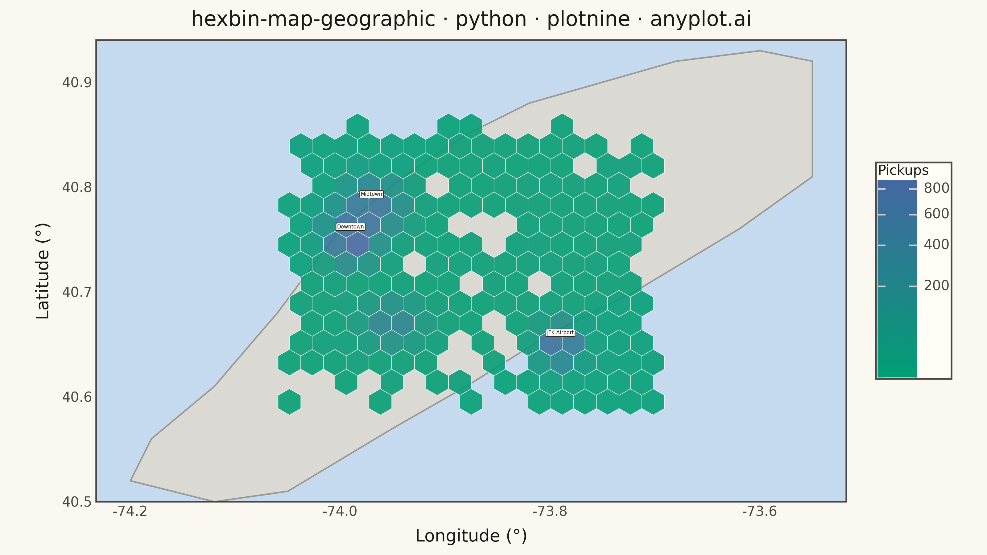
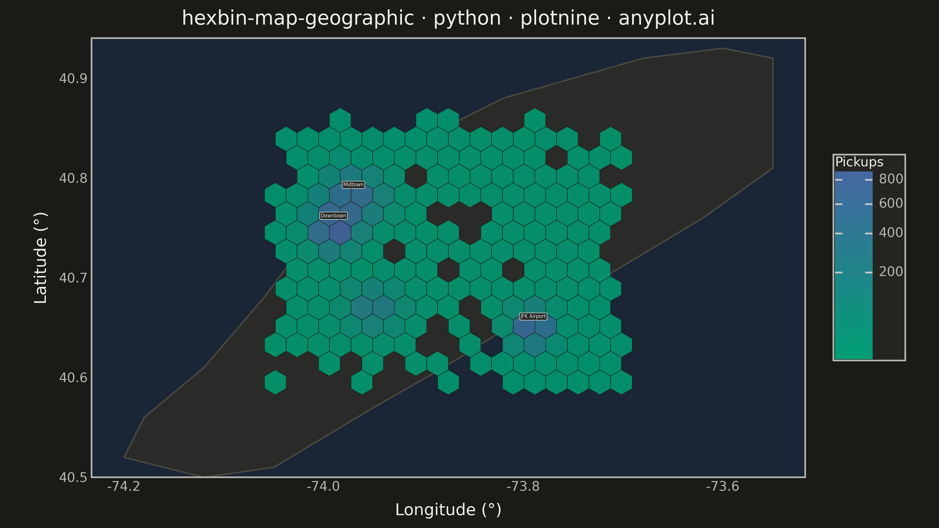
A geographic map visualization that aggregates point data into hexagonal cells, displaying density or aggregated values per cell using color intensity. Unlike continuous heatmaps that use kernel density estimation, hexbin maps provide discrete binning that clearly shows data aggregation boundaries. The hexagonal grid is superior to square grids due to isotropy (equal distance to neighboring cells) and better visual continuity, making it ideal for spatial statistics and urban data analysis.
""" anyplot.ai
hexbin-map-geographic: Hexagonal Binning Map
Library: plotnine 0.15.4 | Python 3.13.13
Quality: 89/100 | Updated: 2026-05-27
"""

import os

import numpy as np
import pandas as pd
from plotnine import (
    aes,
    coord_fixed,
    element_blank,
    element_line,
    element_rect,
    element_text,
    geom_label,
    geom_polygon,
    ggplot,
    labs,
    scale_fill_gradient,
    theme,
    theme_minimal,
)


# Theme tokens
THEME = os.getenv("ANYPLOT_THEME", "light")
PAGE_BG = "#FAF8F1" if THEME == "light" else "#1A1A17"
ELEVATED_BG = "#FFFDF6" if THEME == "light" else "#242420"
INK = "#1A1A17" if THEME == "light" else "#F0EFE8"
INK_SOFT = "#4A4A44" if THEME == "light" else "#B8B7B0"

WATER_COLOR = "#C5D9EF" if THEME == "light" else "#1A2535"
LAND_COLOR = "#DEDAD2" if THEME == "light" else "#2C2C27"
LAND_EDGE = "#9A9A92" if THEME == "light" else "#4A4A42"

# Data — NYC taxi pickup clusters (denser hotspots for full gradient utilization)
np.random.seed(42)

downtown_lon = np.random.normal(-73.99, 0.012, 2500)
downtown_lat = np.random.normal(40.75, 0.010, 2500)

midtown_lon = np.random.normal(-73.97, 0.015, 2200)
midtown_lat = np.random.normal(40.78, 0.012, 2200)

airport_lon = np.random.normal(-73.79, 0.010, 1500)
airport_lat = np.random.normal(40.65, 0.008, 1500)

brooklyn_lon = np.random.normal(-73.95, 0.015, 900)
brooklyn_lat = np.random.normal(40.67, 0.010, 900)

scatter_lon = np.random.uniform(-74.05, -73.70, 400)
scatter_lat = np.random.uniform(40.60, 40.85, 400)

lon = np.concatenate([downtown_lon, midtown_lon, airport_lon, brooklyn_lon, scatter_lon])
lat = np.concatenate([downtown_lat, midtown_lat, airport_lat, brooklyn_lat, scatter_lat])

# Optional value: simulated trip duration (min) — airport trips notably longer
value = np.concatenate(
    [
        np.random.normal(11, 3, 2500),  # downtown — short rides
        np.random.normal(13, 3, 2200),  # midtown
        np.random.normal(38, 6, 1500),  # airport — long rides
        np.random.normal(10, 3, 900),  # brooklyn
        np.random.normal(15, 5, 400),  # scattered
    ]
)

# Hexagonal bin polygon construction
gridsize = 30
LON_MIN, LON_MAX = -74.20, -73.55
LAT_MIN, LAT_MAX = 40.52, 40.92

hex_width = (LON_MAX - LON_MIN) / gridsize
hex_radius = hex_width / np.sqrt(3)
row_height = hex_radius * 1.5

centers = []
row = 0
y_pos = LAT_MIN
while y_pos <= LAT_MAX:
    x_offset = (hex_width / 2) if row % 2 else 0
    x_pos = LON_MIN + x_offset
    while x_pos <= LON_MAX:
        centers.append((x_pos, y_pos))
        x_pos += hex_width
    y_pos += row_height
    row += 1

points = np.column_stack([lon, lat])
records = []
hex_id = 0

for cx, cy in centers:
    dx = np.abs(points[:, 0] - cx)
    dy = np.abs(points[:, 1] - cy)
    in_hex = (
        (dy <= hex_radius)
        & (dx <= hex_width / 2)
        & (hex_radius * hex_width / 2 >= dx * hex_radius + dy * hex_width / 4)
    )
    count = np.sum(in_hex)
    if count > 0:
        mean_value = np.mean(value[in_hex])  # mean aggregation of optional value field
        angles = np.arange(6) * np.pi / 3 + np.pi / 6
        for angle in angles:
            records.append(
                {
                    "lon": cx + hex_radius * np.cos(angle),
                    "lat": cy + hex_radius * np.sin(angle),
                    "hex_id": hex_id,
                    "count": count,
                    "mean_value": mean_value,
                }
            )
        hex_id += 1

hex_df = pd.DataFrame(records)

# Hotspot label positions for direct annotation
labels_df = pd.DataFrame(
    {"lon": [-73.99, -73.97, -73.79], "lat": [40.762, 40.793, 40.661], "label": ["Downtown", "Midtown", "JFK Airport"]}
)

# NYC-like coastline boundary
coast_lon = [
    -74.20,
    -74.12,
    -74.05,
    -74.00,
    -73.95,
    -73.88,
    -73.80,
    -73.72,
    -73.62,
    -73.55,
    -73.55,
    -73.60,
    -73.68,
    -73.75,
    -73.82,
    -73.88,
    -73.94,
    -74.00,
    -74.06,
    -74.12,
    -74.18,
    -74.20,
]
coast_lat = [
    40.52,
    40.50,
    40.51,
    40.54,
    40.57,
    40.61,
    40.66,
    40.70,
    40.76,
    40.81,
    40.92,
    40.93,
    40.92,
    40.90,
    40.88,
    40.85,
    40.81,
    40.76,
    40.68,
    40.61,
    40.56,
    40.52,
]
df_coastline = pd.DataFrame({"region": "land", "order": range(len(coast_lon)), "lon": coast_lon, "lat": coast_lat})

title = "hexbin-map-geographic · python · plotnine · anyplot.ai"

# sqrt transform spreads color across the right-skewed count distribution —
# a ggplot2 grammar-of-graphics feature that replaces manual data normalization
plot = (
    ggplot()
    + geom_polygon(
        aes(x="lon", y="lat", group="region"), data=df_coastline, fill=LAND_COLOR, color=LAND_EDGE, size=0.5, alpha=0.9
    )
    + geom_polygon(
        aes(x="lon", y="lat", group="hex_id", fill="count"), data=hex_df, color=PAGE_BG, size=0.15, alpha=0.88
    )
    + geom_label(
        aes(x="lon", y="lat", label="label"),
        data=labels_df,
        color=INK,
        fill=ELEVATED_BG,
        size=3,
        label_padding=0.2,
        label_size=0.3,
    )
    + scale_fill_gradient(low="#009E73", high="#4467A3", name="Pickups", trans="sqrt")
    + coord_fixed(ratio=1.0, xlim=(-74.20, -73.55), ylim=(40.52, 40.92))
    + labs(title=title, x="Longitude (°)", y="Latitude (°)")
    + theme_minimal()
    + theme(
        figure_size=(8, 4.5),
        plot_background=element_rect(fill=PAGE_BG, color=PAGE_BG),
        panel_background=element_rect(fill=WATER_COLOR),
        panel_border=element_rect(color=INK_SOFT, fill=None),
        panel_grid_major=element_blank(),
        panel_grid_minor=element_blank(),
        plot_title=element_text(size=12, color=INK),
        axis_title=element_text(size=10, color=INK),
        axis_text=element_text(size=8, color=INK_SOFT),
        legend_title=element_text(size=8, color=INK),
        legend_text=element_text(size=8, color=INK_SOFT),
        legend_background=element_rect(fill=ELEVATED_BG, color=INK_SOFT),
        legend_position="right",
        axis_line=element_line(color=INK_SOFT, size=0.3),
    )
)

# Save
plot.save(f"plot-{THEME}.png", dpi=400, width=8, height=4.5, units="in")
Runnable source as JSON, for any HTTP client: https://api.anyplot.ai/specs/hexbin-map-geographic/plotnine/code. Any spec id and library id listed in llms-full.txt fit the same URL shape; every URL below is complete and callable.
{
  "spec_id": "hexbin-map-geographic",
  "language": "python",
  "library": "plotnine",
  "page": "https://anyplot.ai/hexbin-map-geographic/python/plotnine",
  "hub": "https://anyplot.ai/hexbin-map-geographic",
  "code_json": "https://api.anyplot.ai/specs/hexbin-map-geographic/plotnine/code",
  "spec_json": "https://api.anyplot.ai/specs/hexbin-map-geographic",
  "render_light_png": "https://storage.googleapis.com/anyplot-images/plots/hexbin-map-geographic/python/plotnine/plot-light.png",
  "render_dark_png": "https://storage.googleapis.com/anyplot-images/plots/hexbin-map-geographic/python/plotnine/plot-dark.png",
  "quality_score": 89.0,
  "license": "MIT",
  "guide": "https://anyplot.ai/llms.txt"
}
Part of Hexagonal Binning Map on anyplot.ai.