The same plot in 14 other libraries — Python: Altair, Bokeh, lets-plot, Matplotlib, Plotly, plotnine, Pygal, Seaborn; R: ggplot2; JavaScript: Chart.js, D3.js, Apache ECharts, Highcharts, MUI X Charts. Compare all 15 side by side: Hexagonal Binning Map in Python, R, Julia and JavaScript.
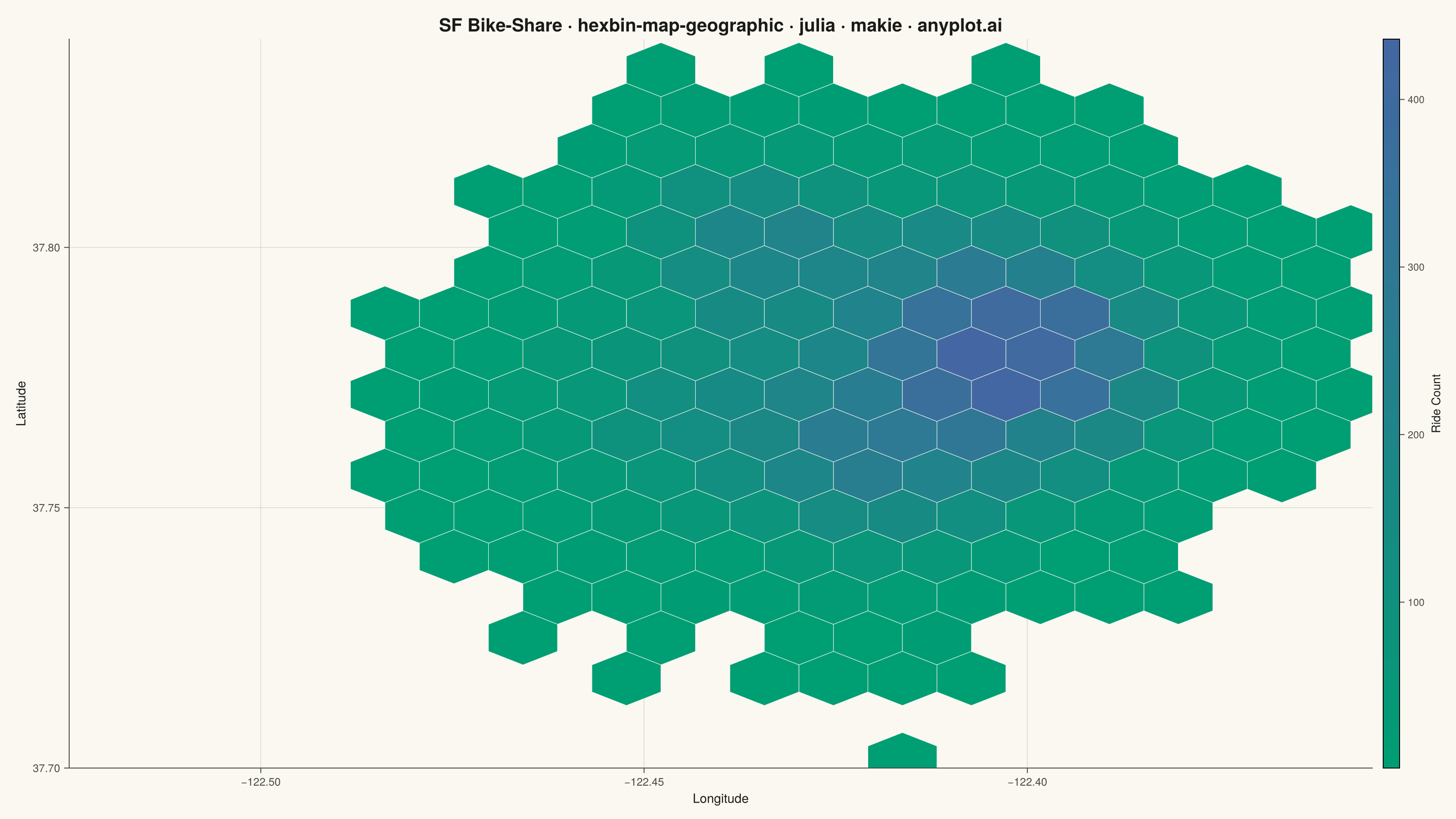
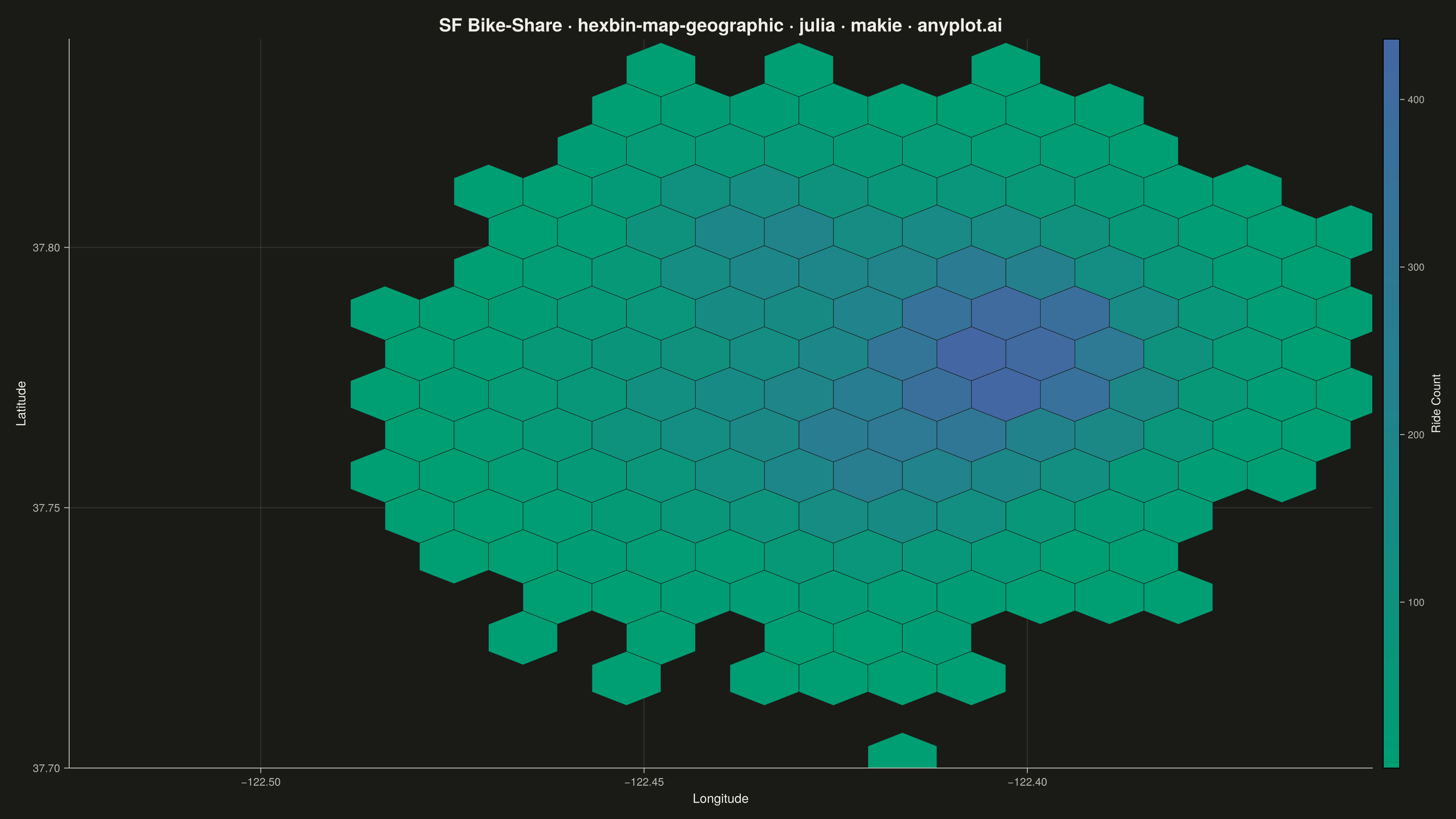
A geographic map visualization that aggregates point data into hexagonal cells, displaying density or aggregated values per cell using color intensity. Unlike continuous heatmaps that use kernel density estimation, hexbin maps provide discrete binning that clearly shows data aggregation boundaries. The hexagonal grid is superior to square grids due to isotropy (equal distance to neighboring cells) and better visual continuity, making it ideal for spatial statistics and urban data analysis.
# anyplot.ai
# hexbin-map-geographic: Hexagonal Binning Map
# Library: makie 0.22.10 | Julia 1.11.9
# Quality: 85/100 | Created: 2026-05-27

using CairoMakie
using Colors
using Random

Random.seed!(42)

# Theme tokens
const THEME       = get(ENV, "ANYPLOT_THEME", "light")
const PAGE_BG     = THEME == "light" ? colorant"#FAF8F1" : colorant"#1A1A17"
const ELEVATED_BG = THEME == "light" ? colorant"#FFFDF6" : colorant"#242420"
const INK         = THEME == "light" ? colorant"#1A1A17" : colorant"#F0EFE8"
const INK_SOFT    = THEME == "light" ? colorant"#4A4A44" : colorant"#B8B7B0"
const INK_MUTED   = THEME == "light" ? colorant"#6B6A63" : colorant"#A8A79F"
const GRID_COLOR  = THEME == "light" ?
    RGBAf(26/255f0, 26/255f0, 23/255f0, 0.12f0) :
    RGBAf(240/255f0, 239/255f0, 232/255f0, 0.12f0)

# Water fill and coastline colors for the geographic base map
const WATER_FILL  = THEME == "light" ?
    RGBAf(0.58f0, 0.75f0, 0.88f0, 0.32f0) :
    RGBAf(0.18f0, 0.35f0, 0.56f0, 0.45f0)
const COAST_LINE  = THEME == "light" ?
    RGBAf(0.27f0, 0.46f0, 0.63f0, 0.65f0) :
    RGBAf(0.42f0, 0.62f0, 0.80f0, 0.52f0)

# Anyplot sequential colormap for density (single-polarity)
const ANYPLOT_SEQ = cgrad([colorant"#009E73", colorant"#4467A3"])

# Data: synthetic bike-share ride starts in San Francisco
cluster_centers = [
    (-122.4057, 37.7871),  # Union Square / Downtown
    (-122.4194, 37.7599),  # Mission District
    (-122.3971, 37.7749),  # SoMa
    (-122.4352, 37.8012),  # Marina
    (-122.4447, 37.7698),  # Haight-Ashbury
]
cluster_weights = [0.33, 0.22, 0.20, 0.13, 0.12]
cluster_stds    = [0.013, 0.012, 0.011, 0.010, 0.013]

n_total = 14000
lons = Float64[]
lats = Float64[]

for ((cx, cy), w, σ) in zip(cluster_centers, cluster_weights, cluster_stds)
    n_i = round(Int, n_total * w)
    append!(lons, cx .+ σ .* randn(n_i))
    append!(lats, cy .+ σ .* randn(n_i))
end

# Map extent — tightened from original to reduce empty ocean space upper-left
lon_lo, lon_hi = -122.515, -122.360
lat_lo, lat_hi =   37.700,   37.835

# Clip to bounds
mask = (lons .>= lon_lo) .& (lons .<= lon_hi) .& (lats .>= lat_lo) .& (lats .<= lat_hi)
lons = lons[mask]
lats = lats[mask]

# --- Simplified geographic base map -----------------------------------------
# Polygon vertices tracing simplified SF coastlines; Makie auto-closes last→first.

# SF Bay water polygon: follows the eastern SF waterfront (south→north),
# then closes via the box top-right corner and right edge.
bay_pts = Point2f[
    (-122.374, 37.700), (-122.376, 37.748), (-122.381, 37.762),
    (-122.386, 37.776), (-122.393, 37.790), (-122.400, 37.800),
    (-122.407, 37.805), (-122.414, 37.808), (-122.432, 37.804),
    (-122.443, 37.803), (-122.455, 37.803), (-122.464, 37.804),
    (-122.479, 37.808),                       # Golden Gate Bridge — SF side
    (-122.479, 37.835), (-122.360, 37.835), (-122.360, 37.700),
]

# Pacific Ocean polygon: follows the western SF coast (north→south),
# then closes via the box bottom-left and left edge back to the top.
pac_pts = Point2f[
    (-122.479, 37.808),                       # Golden Gate Bridge — SF side
    (-122.484, 37.800), (-122.493, 37.798),
    (-122.499, 37.794), (-122.505, 37.789),
    (-122.509, 37.782), (-122.511, 37.770),
    (-122.512, 37.748), (-122.511, 37.710),
    (-122.515, 37.700), (-122.515, 37.835),
    (-122.479, 37.835),
]

# --- Figure -----------------------------------------------------------------
fig = Figure(
    size            = (1600, 900),
    fontsize        = 14,
    backgroundcolor = PAGE_BG,
)

ax = Axis(
    fig[1, 1];
    title              = "SF Bike-Share · hexbin-map-geographic · julia · makie · anyplot.ai",
    titlesize          = 20,
    titlecolor         = INK,
    xlabel             = "Longitude",
    ylabel             = "Latitude",
    xlabelsize         = 14,
    ylabelsize         = 14,
    xticklabelsize     = 12,
    yticklabelsize     = 12,
    xlabelcolor        = INK,
    ylabelcolor        = INK,
    xticklabelcolor    = INK_SOFT,
    yticklabelcolor    = INK_SOFT,
    xtickcolor         = INK_SOFT,
    ytickcolor         = INK_SOFT,
    backgroundcolor    = PAGE_BG,
    topspinevisible    = false,
    rightspinevisible  = false,
    leftspinecolor     = INK_SOFT,
    bottomspinecolor   = INK_SOFT,
    xgridcolor         = GRID_COLOR,
    ygridcolor         = GRID_COLOR,
    xminorgridvisible  = false,
    yminorgridvisible  = false,
)

# Base map: water bodies rendered before hexbins so land clusters stay visible
poly!(ax, bay_pts; color = WATER_FILL, strokecolor = COAST_LINE, strokewidth = 1.2)
poly!(ax, pac_pts; color = WATER_FILL, strokecolor = COAST_LINE, strokewidth = 1.2)

# Hexagonal density map overlaid on base map
hb = hexbin!(ax, lons, lats;
    cellsize    = 0.009,
    colormap    = ANYPLOT_SEQ,
    threshold   = 1,
    strokecolor = PAGE_BG,
    strokewidth = 0.5,
)

# Colorbar
Colorbar(fig[1, 2], hb;
    label           = "Ride Count",
    labelsize       = 13,
    labelcolor      = INK,
    ticklabelsize   = 11,
    ticklabelcolor  = INK_SOFT,
    tickcolor       = INK_SOFT,
    width           = 18,
)

limits!(ax, lon_lo, lon_hi, lat_lo, lat_hi)
colgap!(fig.layout, 12)

save("plot-$(THEME).png", fig; px_per_unit = 2)
Runnable source as JSON, for any HTTP client: https://api.anyplot.ai/specs/hexbin-map-geographic/makie/code. Any spec id and library id listed in llms-full.txt fit the same URL shape; every URL below is complete and callable.
{
  "spec_id": "hexbin-map-geographic",
  "language": "julia",
  "library": "makie",
  "page": "https://anyplot.ai/hexbin-map-geographic/julia/makie",
  "hub": "https://anyplot.ai/hexbin-map-geographic",
  "code_json": "https://api.anyplot.ai/specs/hexbin-map-geographic/makie/code",
  "spec_json": "https://api.anyplot.ai/specs/hexbin-map-geographic",
  "render_light_png": "https://storage.googleapis.com/anyplot-images/plots/hexbin-map-geographic/julia/makie/plot-light.png",
  "render_dark_png": "https://storage.googleapis.com/anyplot-images/plots/hexbin-map-geographic/julia/makie/plot-dark.png",
  "quality_score": 85.0,
  "license": "MIT",
  "guide": "https://anyplot.ai/llms.txt"
}
Part of Hexagonal Binning Map on anyplot.ai.