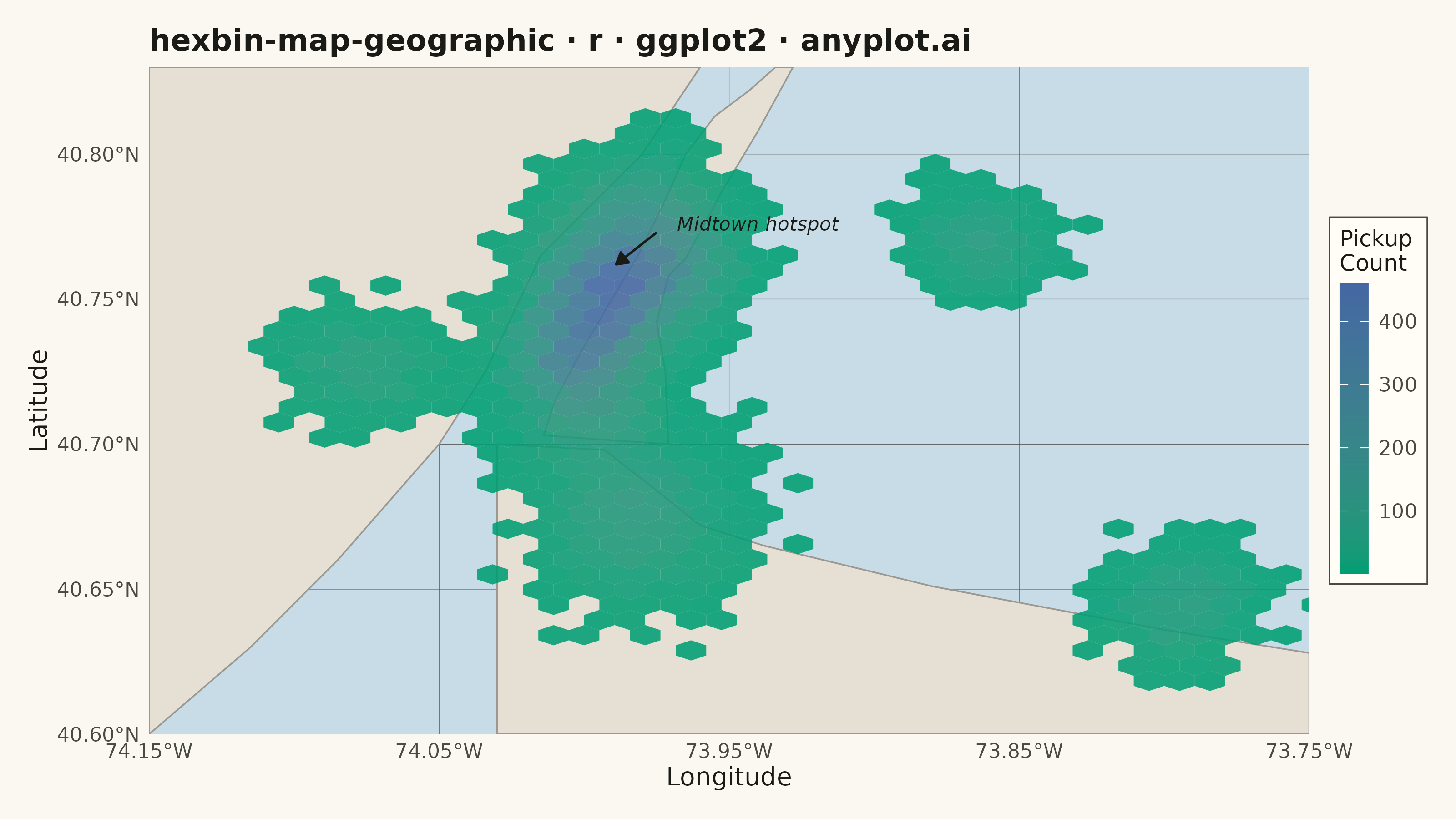
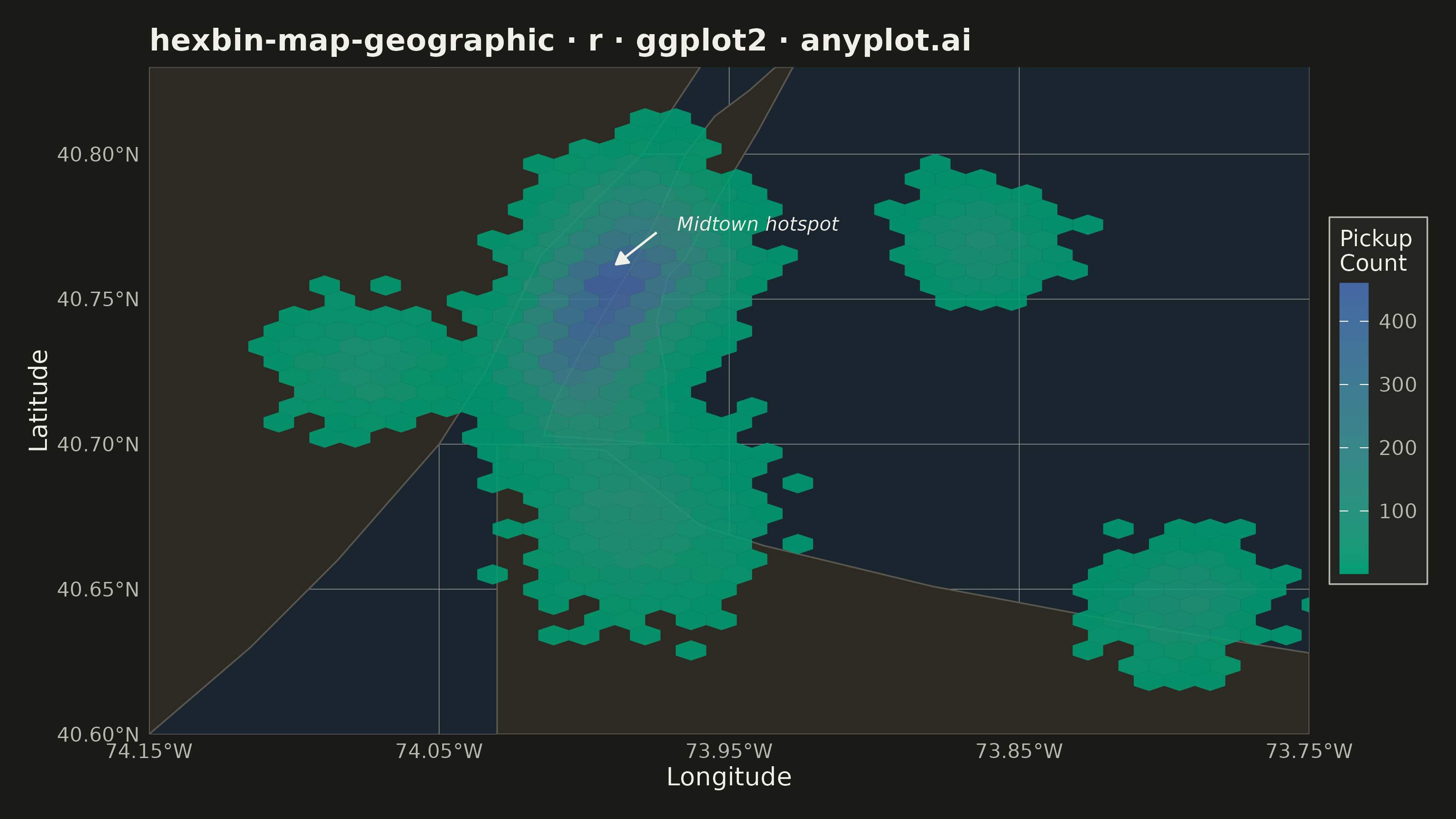
The same plot in 14 other libraries — Python: Altair, Bokeh, lets-plot, Matplotlib, Plotly, plotnine, Pygal, Seaborn; Julia: Makie.jl; JavaScript: Chart.js, D3.js, Apache ECharts, Highcharts, MUI X Charts. Compare all 15 side by side: Hexagonal Binning Map in Python, R, Julia and JavaScript.
A geographic map visualization that aggregates point data into hexagonal cells, displaying density or aggregated values per cell using color intensity. Unlike continuous heatmaps that use kernel density estimation, hexbin maps provide discrete binning that clearly shows data aggregation boundaries. The hexagonal grid is superior to square grids due to isotropy (equal distance to neighboring cells) and better visual continuity, making it ideal for spatial statistics and urban data analysis.
#' anyplot.ai
#' hexbin-map-geographic: Hexagonal Binning Map
#' Library: ggplot2 3.5.1 | R 4.4.1
#' Quality: 89/100 | Created: 2026-05-27

library(ggplot2)
library(dplyr)
library(tibble)
library(scales)
library(ragg)

set.seed(42)

# Theme tokens
THEME       <- Sys.getenv("ANYPLOT_THEME", "light")
PAGE_BG     <- if (THEME == "light") "#FAF8F1" else "#1A1A17"
ELEVATED_BG <- if (THEME == "light") "#FFFDF6" else "#242420"
INK         <- if (THEME == "light") "#1A1A17" else "#F0EFE8"
INK_SOFT    <- if (THEME == "light") "#4A4A44" else "#B8B7B0"
MAP_WATER   <- if (THEME == "light") "#C8DCE8" else "#1A2530"
MAP_LAND    <- if (THEME == "light") "#E6E0D4" else "#2C2A22"
MAP_BORDER  <- if (THEME == "light") "#9A9890" else "#58584E"

# NYC metro area taxi pickups — simulated density clusters
# Centres: Midtown, Greenwich Village, UWS, Chelsea, S.Brooklyn,
#          Midtown East, Lower Manhattan, JFK-adjacent, LGA-adjacent, Jersey City
cluster_centers <- tibble::tibble(
  lat   = c(40.756, 40.730, 40.775, 40.744, 40.676,
             40.762, 40.710, 40.645, 40.769, 40.727),
  lon   = c(-73.989, -74.003, -73.981, -73.995, -73.982,
             -73.971, -73.997, -73.794, -73.863, -74.077),
  n     = c(5000L, 3200L, 2400L, 2600L, 1800L,
             1400L, 1000L, 700L, 600L, 500L),
  s_lat = c(0.010, 0.009, 0.011, 0.009, 0.013,
             0.010, 0.009, 0.009, 0.008, 0.009),
  s_lon = c(0.013, 0.011, 0.013, 0.011, 0.015,
             0.012, 0.011, 0.012, 0.010, 0.011)
)

pickups <- dplyr::bind_rows(
  lapply(seq_len(nrow(cluster_centers)), function(i) {
    cc <- cluster_centers[i, ]
    tibble::tibble(
      lat = rnorm(cc$n, cc$lat, cc$s_lat),
      lon = rnorm(cc$n, cc$lon, cc$s_lon)
    )
  })
) |> dplyr::filter(
  lat >= 40.60, lat <= 40.83,
  lon >= -74.15, lon <= -73.75
)

# --- Simplified NYC geographic context (hand-digitized approximate outlines) ---
# sf/rnaturalearth not available; inline polygons provide coastline context.
# Water shows as panel background (MAP_WATER).

# New Jersey — land mass west of the Hudson River
nj_land <- tibble::tibble(
  group = "nj",
  lon   = c(-74.15, -74.15, -73.960, -73.980, -74.015, -74.034, -74.050,
            -74.085, -74.115, -74.15),
  lat   = c(40.60,  40.83,  40.830,  40.800,  40.765,  40.725,  40.700,
            40.660,  40.630,  40.60)
)

# Manhattan Island — narrow north-south strip between Hudson and East River.
# Points trace the eastern shoreline (Battery → Harlem) then west (Harlem → Battery).
manhattan_land <- tibble::tibble(
  group = "manhattan",
  lon   = c(
    # East shore: south to north
    -73.971, -73.972, -73.975, -73.971, -73.965, -73.952, -73.940, -73.928,
    # North clip at lat 40.830 (Inwood not in view)
    -73.934, -73.943,
    # West shore: north to south
    -73.955, -73.965, -73.973, -73.982, -73.991, -74.001, -74.010, -74.014, -73.971
  ),
  lat   = c(
    40.700, 40.725, 40.742, 40.758, 40.764, 40.788, 40.808, 40.830,
    40.830, 40.822,
    40.813, 40.800, 40.782, 40.764, 40.749, 40.732, 40.715, 40.703, 40.700
  )
)

# Brooklyn and Queens — southeastern land mass south of the East River
bq_land <- tibble::tibble(
  group = "bq",
  lon   = c(-74.030, -73.993, -73.975, -73.960, -73.938, -73.880, -73.800,
            -73.75,  -73.75,  -74.030),
  lat   = c(40.700,  40.698,  40.684,  40.672,  40.665,  40.651,  40.636,
            40.628,  40.60,   40.60)
)

nyc_geo <- dplyr::bind_rows(nj_land, manhattan_land, bq_land)

# --- Plot ---

plot_title <- "hexbin-map-geographic · r · ggplot2 · anyplot.ai"
title_size <- max(8L, round(12 * min(1.0, 67 / nchar(plot_title))))

p <- ggplot() +
  # Geographic base map
  geom_polygon(
    data      = nyc_geo,
    aes(x = lon, y = lat, group = group),
    fill      = MAP_LAND,
    color     = MAP_BORDER,
    linewidth = 0.30
  ) +
  # Hexbin density layer
  geom_hex(
    data  = pickups,
    aes(x = lon, y = lat),
    bins  = 38,
    alpha = 0.88
  ) +
  # Storytelling annotation: point to primary hotspot
  annotate("segment",
    x = -73.975, xend = -73.989,
    y = 40.773,  yend = 40.762,
    color = INK, linewidth = 0.45,
    arrow = arrow(length = unit(0.18, "cm"), type = "closed")
  ) +
  annotate("text",
    x = -73.968, y = 40.776,
    label    = "Midtown hotspot",
    color    = INK,
    size     = 2.7,
    fontface = "italic",
    hjust    = 0
  ) +
  scale_fill_gradient(
    low    = "#009E73",
    high   = "#4467A3",
    name   = "Pickup\nCount",
    labels = scales::comma,
    guide  = guide_colorbar(barwidth = 0.8, barheight = 8)
  ) +
  scale_x_continuous(
    labels = function(x) sprintf("%.2f°W", -x),
    expand = expansion(mult = 0.0)
  ) +
  scale_y_continuous(
    labels = function(y) sprintf("%.2f°N", y),
    expand = expansion(mult = 0.0)
  ) +
  coord_fixed(
    ratio = 1,
    xlim  = c(-74.15, -73.75),
    ylim  = c(40.60, 40.83)
  ) +
  labs(
    x     = "Longitude",
    y     = "Latitude",
    title = plot_title
  ) +
  theme_minimal(base_size = 8) +
  theme(
    plot.background   = element_rect(fill = PAGE_BG, color = PAGE_BG),
    panel.background  = element_rect(fill = MAP_WATER, color = NA),
    panel.grid.major  = element_line(color = INK_SOFT, linewidth = 0.10),
    panel.grid.minor  = element_blank(),
    axis.title        = element_text(color = INK,      size = 10),
    axis.text         = element_text(color = INK_SOFT, size = 8),
    plot.title        = element_text(color = INK,      size = title_size, face = "bold"),
    legend.background = element_rect(fill = ELEVATED_BG, color = INK_SOFT, linewidth = 0.3),
    legend.text       = element_text(color = INK_SOFT, size = 8),
    legend.title      = element_text(color = INK,      size = 9),
    legend.position   = "right",
    plot.margin       = margin(0.4, 0.4, 0.4, 0.4, "cm")
  )

ggsave(
  filename = sprintf("plot-%s.png", THEME),
  plot     = p,
  device   = ragg::agg_png,
  width    = 8,
  height   = 4.5,
  units    = "in",
  dpi      = 400
)
Runnable source as JSON, for any HTTP client: https://api.anyplot.ai/specs/hexbin-map-geographic/ggplot2/code. Any spec id and library id listed in llms-full.txt fit the same URL shape; every URL below is complete and callable.
{
  "spec_id": "hexbin-map-geographic",
  "language": "r",
  "library": "ggplot2",
  "page": "https://anyplot.ai/hexbin-map-geographic/r/ggplot2",
  "hub": "https://anyplot.ai/hexbin-map-geographic",
  "code_json": "https://api.anyplot.ai/specs/hexbin-map-geographic/ggplot2/code",
  "spec_json": "https://api.anyplot.ai/specs/hexbin-map-geographic",
  "render_light_png": "https://storage.googleapis.com/anyplot-images/plots/hexbin-map-geographic/r/ggplot2/plot-light.png",
  "render_dark_png": "https://storage.googleapis.com/anyplot-images/plots/hexbin-map-geographic/r/ggplot2/plot-dark.png",
  "quality_score": 89.0,
  "license": "MIT",
  "guide": "https://anyplot.ai/llms.txt"
}
Part of Hexagonal Binning Map on anyplot.ai.