The same plot in 14 other libraries — JavaScript: Chart.js, D3.js, Apache ECharts, Highcharts; Python: Altair, Bokeh, lets-plot, Matplotlib, Plotly, plotnine, Pygal, Seaborn; R: ggplot2; Julia: Makie.jl. Compare all 15 side by side: Hexagonal Binning Map in Python, R, Julia and JavaScript.
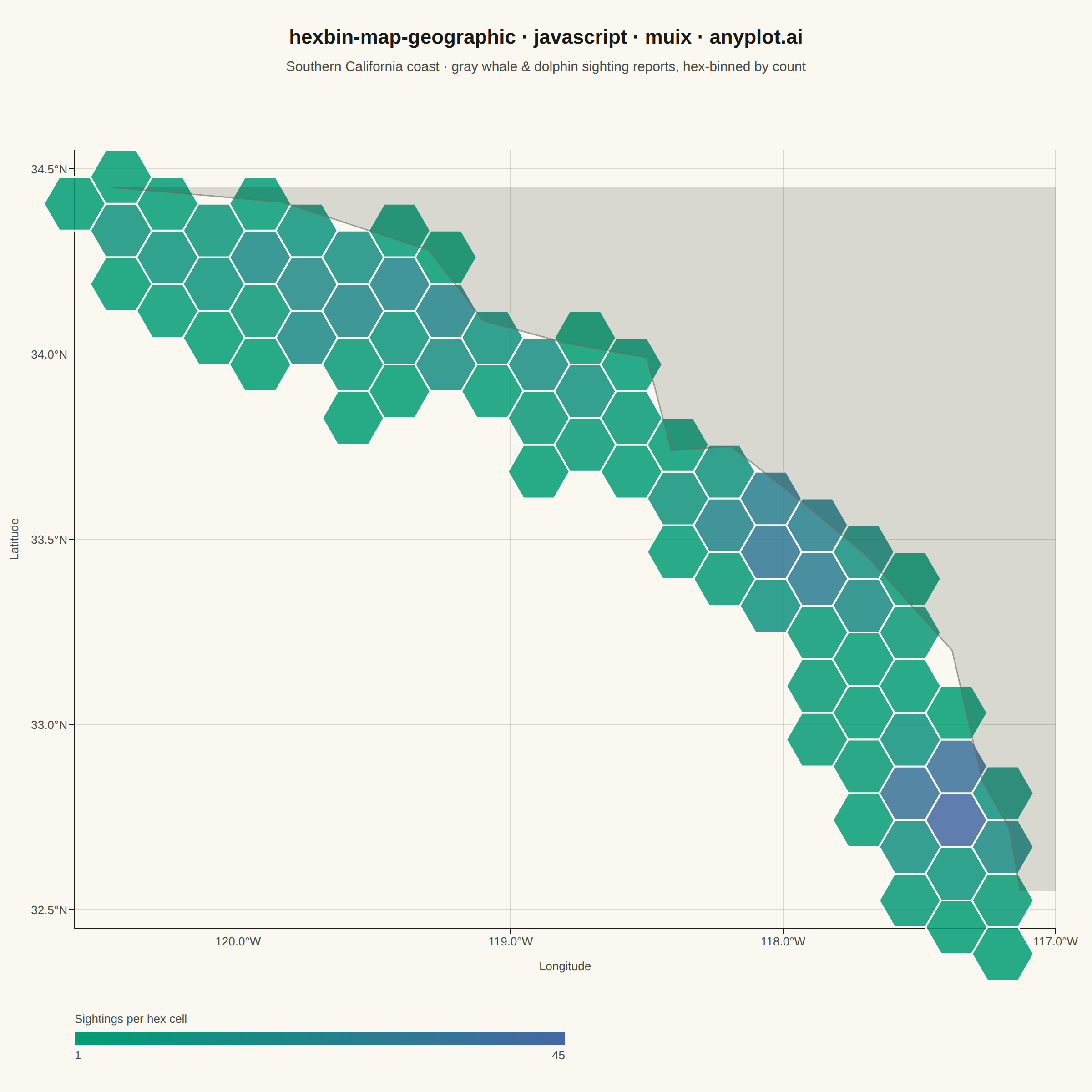
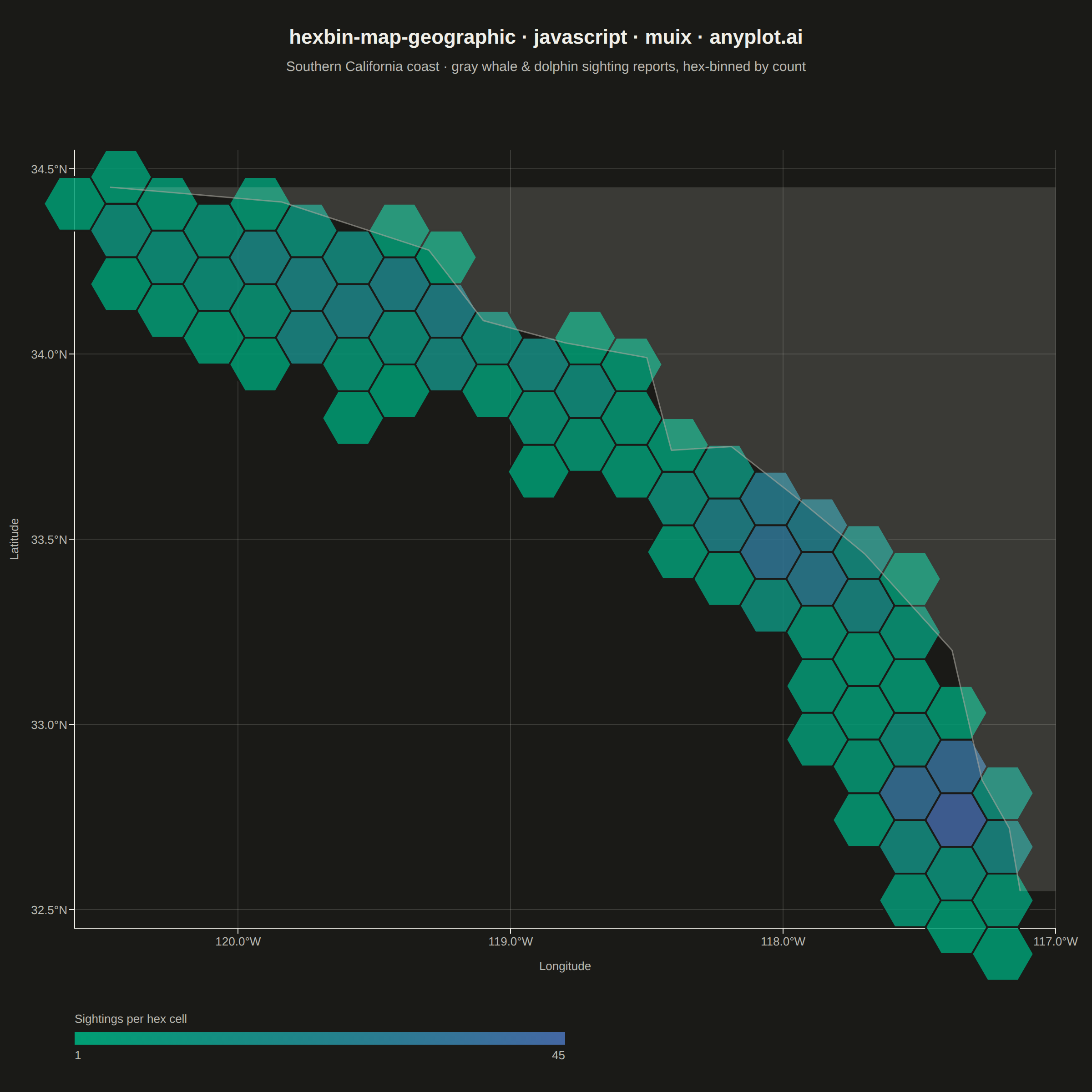
A geographic map visualization that aggregates point data into hexagonal cells, displaying density or aggregated values per cell using color intensity. Unlike continuous heatmaps that use kernel density estimation, hexbin maps provide discrete binning that clearly shows data aggregation boundaries. The hexagonal grid is superior to square grids due to isotropy (equal distance to neighboring cells) and better visual continuity, making it ideal for spatial statistics and urban data analysis.
// anyplot.ai
// hexbin-map-geographic: Hexagonal Binning Map
// Library: muix 7.29.1 | JavaScript 22.23.2
// Quality: 90/100 | Created: 2026-08-25
//# anyplot-orientation: square
// anyplot.ai
// hexbin-map-geographic: Whale & Dolphin Sighting Density, Southern California Coast
// Library: MUI X Charts | React | Node 22
// License: @mui/x-charts — MIT (community). Pro/Premium are out of scope.
// Quality: pending | Created: 2026-08-25
import { ScatterChart } from "@mui/x-charts/ScatterChart";
import { useXScale, useYScale } from "@mui/x-charts/hooks";
const t = window.ANYPLOT_TOKENS;
const THEME = window.ANYPLOT_THEME === "dark" ? "dark" : "light";
const INK_MUTED = THEME === "dark" ? "#A8A79F" : "#6B6A63";
// --- Geographic domain: Southern California coast, Point Conception to San
// Diego. The community @mui/x-charts surface has no polygon/basemap
// primitive, so lon/lat are plotted directly as linear axes (a simple
// equirectangular projection) and the coastline is hand-traced from ~14
// approximate real vertices via the chart's own xScale/yScale hooks — the
// same technique used to place any custom SVG overlay on a MUI X chart. ----
const LON_MIN = -120.6;
const LON_MAX = -117.0;
const LAT_MIN = 32.45;
const LAT_MAX = 34.55;
// North -> south, approximate real coastline vertices (degrees).
const COASTLINE = [
[-120.47, 34.45], // Point Conception
[-119.84, 34.41], // Santa Barbara
[-119.3, 34.28], // Ventura
[-119.1, 34.09], // Point Mugu
[-118.8, 34.03], // Malibu
[-118.5, 33.99], // Santa Monica
[-118.41, 33.74], // Palos Verdes
[-118.19, 33.75], // Long Beach
[-117.93, 33.6], // Newport Beach
[-117.7, 33.46], // Dana Point
[-117.38, 33.2], // Oceanside
[-117.27, 32.85], // La Jolla
[-117.17, 32.72], // San Diego Bay
[-117.13, 32.55], // Point Loma
];
// --- Deterministic PRNG (mulberry32) — the browser has no seeded RNG ------
let seed = 42;
function rand() {
seed |= 0;
seed = (seed + 0x6d2b79f5) | 0;
let x = Math.imul(seed ^ (seed >>> 15), 1 | seed);
x = (x + Math.imul(x ^ (x >>> 7), 61 | x)) ^ x;
return ((x ^ (x >>> 14)) >>> 0) / 4294967296;
}
function gaussian() {
const u = Math.max(rand(), 1e-9);
const v = rand();
return Math.sqrt(-2 * Math.log(u)) * Math.cos(2 * Math.PI * v);
}
// Coastline longitude at a given latitude, by linear interpolation between
// the traced vertices — used to keep synthetic sightings offshore.
function coastLonAt(lat) {
for (let i = 0; i < COASTLINE.length - 1; i += 1) {
const [lonA, latA] = COASTLINE[i];
const [lonB, latB] = COASTLINE[i + 1];
if ((lat <= latA && lat >= latB) || (lat >= latA && lat <= latB)) {
const f = (lat - latA) / (latB - latA);
return lonA + f * (lonB - lonA);
}
}
// Outside the traced range: snap to whichever end (north/Point Conception
// or south/Point Loma) is actually closest, not always the last vertex.
return lat > COASTLINE[0][1] ? COASTLINE[0][0] : COASTLINE[COASTLINE.length - 1][0];
}
// --- Data: synthetic gray-whale & common-dolphin sighting reports, clustered
// around three real Southern California whale-watching launch points and
// offset west of the coast into open water, plus sparse background sightings
// along the rest of the coastline. -------------------------------------------
const HOTSPOTS = [
{ lat: 34.15, lonOffset: 0.55, sigma: 0.28, n: 260 }, // Santa Barbara Channel / Channel Islands
{ lat: 33.47, lonOffset: 0.22, sigma: 0.16, n: 190 }, // Dana Point
{ lat: 32.78, lonOffset: 0.18, sigma: 0.14, n: 170 }, // La Jolla / San Diego
];
const points = [];
HOTSPOTS.forEach(({ lat: centerLat, lonOffset, sigma, n }) => {
for (let i = 0; i < n; i += 1) {
const lat = centerLat + gaussian() * sigma * 0.6;
const coastLon = coastLonAt(lat);
const lon = coastLon - Math.abs(lonOffset + gaussian() * sigma);
if (lon > LON_MIN && lon < LON_MAX - 0.05 && lat > LAT_MIN && lat < LAT_MAX) {
points.push([lon, lat]);
}
}
});
for (let i = 0; i < 140; i += 1) {
const lat = LAT_MIN + rand() * (LAT_MAX - LAT_MIN);
const coastLon = coastLonAt(lat);
const lon = coastLon - 0.05 - rand() * 0.5;
if (lon > LON_MIN) points.push([lon, lat]);
}
// --- Hexagonal binning, done in PIXEL space (after projection) so the drawn
// cells are always regular hexagons and bin adjacency is isotropic — equal
// screen distance to every neighbor, the property that makes hex grids
// superior to square grids for spatial aggregation. --------------------------
const { width, height } = window.ANYPLOT_SIZE;
const margin = { top: 165, right: 40, bottom: 180, left: 82 };
const innerWidth = width - margin.left - margin.right;
const innerHeight = height - margin.top - margin.bottom;
const lonToPx = (lon) => margin.left + ((lon - LON_MIN) / (LON_MAX - LON_MIN)) * innerWidth;
const latToPy = (lat) => margin.top + (1 - (lat - LAT_MIN) / (LAT_MAX - LAT_MIN)) * innerHeight;
const pxToLon = (px) => LON_MIN + ((px - margin.left) / innerWidth) * (LON_MAX - LON_MIN);
const pyToLat = (py) => LAT_MIN + (1 - (py - margin.top) / innerHeight) * (LAT_MAX - LAT_MIN);
const HEX_R = 34; // center-to-vertex radius, in CSS px
// Cube-round a fractional axial coordinate to its nearest hex (redblobgames).
function axialRound(q, r) {
const x = q;
const z = r;
const y = -x - z;
let rx = Math.round(x);
let ry = Math.round(y);
let rz = Math.round(z);
const xDiff = Math.abs(rx - x);
const yDiff = Math.abs(ry - y);
const zDiff = Math.abs(rz - z);
if (xDiff > yDiff && xDiff > zDiff) rx = -ry - rz;
else if (yDiff > zDiff) ry = -rx - rz;
else rz = -rx - ry;
return [rx, rz];
}
const binMap = new Map();
points.forEach(([lon, lat]) => {
const px = lonToPx(lon) - margin.left;
const py = latToPy(lat) - margin.top;
const q = (2 / 3) * (px / HEX_R);
const r = (-1 / 3) * (px / HEX_R) + (Math.sqrt(3) / 3) * (py / HEX_R);
const [rq, rr] = axialRound(q, r);
const key = `${rq},${rr}`;
binMap.set(key, (binMap.get(key) || 0) + 1);
});
const bins = Array.from(binMap.entries()).map(([key, count]) => {
const [q, r] = key.split(",").map(Number);
const cx = margin.left + HEX_R * 1.5 * q;
const cy = margin.top + HEX_R * Math.sqrt(3) * (r + q / 2);
return { count, cx, cy, lon: pxToLon(cx), lat: pyToLat(cy) };
});
const maxCount = Math.max(2, ...bins.map((b) => b.count));
const series = [
{
id: "hex-bins",
label: "Sighting density",
data: bins.map((b, i) => ({ x: b.lon, y: b.lat, id: `hex-${i}` })),
markerSize: HEX_R,
color: t.palette[0],
valueFormatter: (_value, context) => {
const b = bins[context.dataIndex];
const lonLabel = `${Math.abs(b.lon).toFixed(2)}°W`;
const latLabel = `${b.lat.toFixed(2)}°N`;
return `${b.count} sighting${b.count === 1 ? "" : "s"} · ${lonLabel}, ${latLabel}`;
},
},
];
// --- Custom scatter-marker slot: renders each bin as a flat-top hexagon
// (instead of MUI X's default circle), fill color driven by the zAxis
// colorMap below. Hover/tooltip still work — they key off the underlying
// data point positions, independent of how the marker is drawn. ------------
function HexMarks({ series: s, xScale, yScale, markerSize, color, colorGetter }) {
return (
<g>
{s.data.map((d, i) => {
if (d === null) return null;
const cx = xScale(d.x);
const cy = yScale(d.y);
const fill = colorGetter ? colorGetter(i) : color;
const hexPoints = Array.from({ length: 6 }, (_, k) => {
const angle = (Math.PI / 180) * (60 * k);
return `${cx + markerSize * Math.cos(angle)},${cy + markerSize * Math.sin(angle)}`;
}).join(" ");
return <polygon key={d.id ?? i} points={hexPoints} fill={fill} fillOpacity={0.85} stroke={t.pageBg} strokeWidth={2} />;
})}
</g>
);
}
// Simplified coastline + land tint, positioned via the chart's real scales.
function CoastlineLayer() {
const xScale = useXScale();
const yScale = useYScale();
const coastPx = COASTLINE.map(([lon, lat]) => [xScale(lon), yScale(lat)]);
const top = coastPx[0];
const bottom = coastPx[coastPx.length - 1];
const landPolygon = [[xScale(LON_MAX), top[1]], ...coastPx, [xScale(LON_MAX), bottom[1]]].map((p) => p.join(",")).join(" ");
const coastPath = coastPx.map((p, i) => `${i === 0 ? "M" : "L"} ${p[0]} ${p[1]}`).join(" ");
return (
<g>
<polygon points={landPolygon} fill={t.grid} />
<path d={coastPath} fill="none" stroke={INK_MUTED} strokeWidth={1.5} strokeOpacity={0.6} />
</g>
);
}
const title = "hexbin-map-geographic · javascript · muix · anyplot.ai";
const titleFontSize = Math.round(22 * Math.min(1, 67 / title.length));
// Continuous density legend — @mui/x-charts has no built-in colorbar for a
// zAxis colorMap, so it's drawn with plain SVG using the same imprint_seq
// stops passed to the chart.
function DensityLegend() {
const legendX = margin.left;
const legendY = height - 66;
const legendWidth = innerWidth * 0.5;
return (
<g>
<defs>
<linearGradient id="densityGradient" x1="0" x2="1" y1="0" y2="0">
<stop offset="0" stopColor={t.seq[0]} />
<stop offset="1" stopColor={t.seq[1]} />
</linearGradient>
</defs>
<text x={legendX} y={legendY - 10} fontSize={13} fill={t.inkSoft}>
Sightings per hex cell
</text>
<rect x={legendX} y={legendY} width={legendWidth} height={14} fill="url(#densityGradient)" />
<text x={legendX} y={legendY + 30} fontSize={13} fill={t.inkSoft}>
1
</text>
<text x={legendX + legendWidth} y={legendY + 30} textAnchor="end" fontSize={13} fill={t.inkSoft}>
{maxCount}
</text>
</g>
);
}
// --- Chart (default-exported component — the harness mounts it) -----------
export default function Chart() {
return (
<ScatterChart
width={width}
height={height}
series={series}
zAxis={[
{ data: bins.map((b) => b.count), colorMap: { type: "continuous", min: 1, max: maxCount, color: [t.seq[0], t.seq[1]] } },
]}
margin={margin}
xAxis={[
{
scaleType: "linear",
min: LON_MIN,
max: LON_MAX,
tickNumber: 5,
valueFormatter: (v) => `${Math.abs(v).toFixed(1)}°W`,
tickLabelStyle: { fontSize: 13, fill: t.inkSoft },
},
]}
yAxis={[
{
scaleType: "linear",
min: LAT_MIN,
max: LAT_MAX,
tickNumber: 5,
valueFormatter: (v) => `${v.toFixed(1)}°N`,
tickLabelStyle: { fontSize: 13, fill: t.inkSoft },
},
]}
grid={{ vertical: true, horizontal: true }}
slots={{ scatter: HexMarks }}
tooltip={{ trigger: "item" }}
legend={{ hidden: true }}
skipAnimation
>
<CoastlineLayer />
<text x={width / 2} y={48} textAnchor="middle" fontSize={titleFontSize} fontWeight={600} fill={t.ink}>
{title}
</text>
<text x={width / 2} y={78} textAnchor="middle" fontSize={15} fill={t.inkSoft}>
Southern California coast · gray whale & dolphin sighting reports, hex-binned by count
</text>
<text x={margin.left + innerWidth / 2} y={height - margin.bottom + 46} textAnchor="middle" fontSize={13} fill={t.inkSoft}>
Longitude
</text>
<text
x={20}
y={margin.top + innerHeight / 2}
textAnchor="middle"
fontSize={13}
fill={t.inkSoft}
transform={`rotate(-90 20 ${margin.top + innerHeight / 2})`}
>
Latitude
</text>
<DensityLegend />
</ScatterChart>
);
}
Runnable source as JSON, for any HTTP client: https://api.anyplot.ai/specs/hexbin-map-geographic/muix/code. Any spec id and library id listed in llms-full.txt fit the same URL shape; every URL below is complete and callable.
{
  "spec_id": "hexbin-map-geographic",
  "language": "javascript",
  "library": "muix",
  "page": "https://anyplot.ai/hexbin-map-geographic/javascript/muix",
  "hub": "https://anyplot.ai/hexbin-map-geographic",
  "code_json": "https://api.anyplot.ai/specs/hexbin-map-geographic/muix/code",
  "spec_json": "https://api.anyplot.ai/specs/hexbin-map-geographic",
  "render_light_png": "https://storage.googleapis.com/anyplot-images/plots/hexbin-map-geographic/javascript/muix/plot-light.png",
  "render_dark_png": "https://storage.googleapis.com/anyplot-images/plots/hexbin-map-geographic/javascript/muix/plot-dark.png",
  "interactive_light_html": "https://storage.googleapis.com/anyplot-images/plots/hexbin-map-geographic/javascript/muix/plot-light.html",
  "interactive_dark_html": "https://storage.googleapis.com/anyplot-images/plots/hexbin-map-geographic/javascript/muix/plot-dark.html",
  "quality_score": 90.0,
  "license": "MIT",
  "guide": "https://anyplot.ai/llms.txt"
}
Part of Hexagonal Binning Map on anyplot.ai.