The same plot in 14 other libraries — Python: Bokeh, lets-plot, Matplotlib, Plotly, plotnine, Pygal, Seaborn; R: ggplot2; Julia: Makie.jl; JavaScript: Chart.js, D3.js, Apache ECharts, Highcharts, MUI X Charts. Compare all 15 side by side: Hexagonal Binning Map in Python, R, Julia and JavaScript.
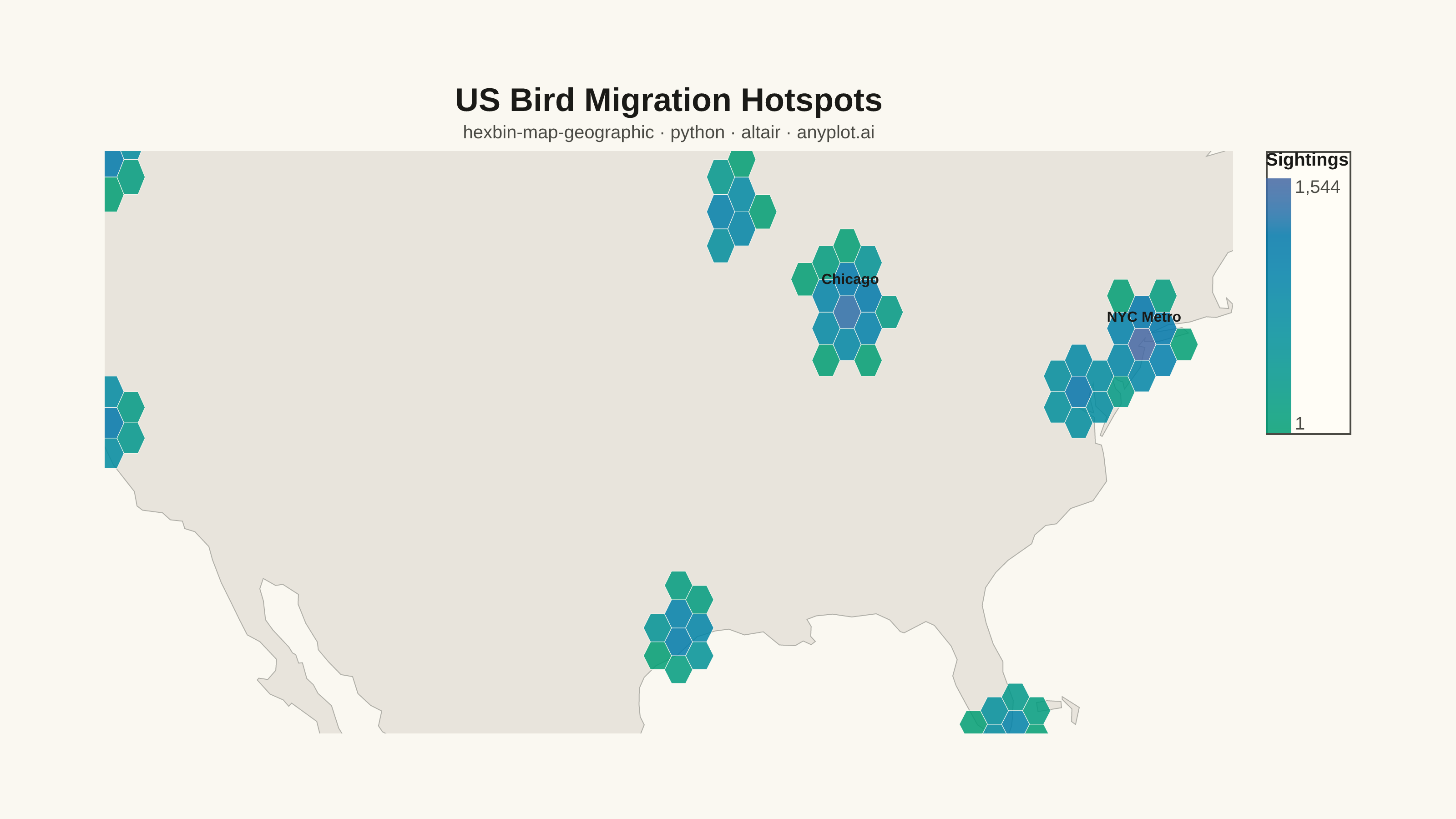
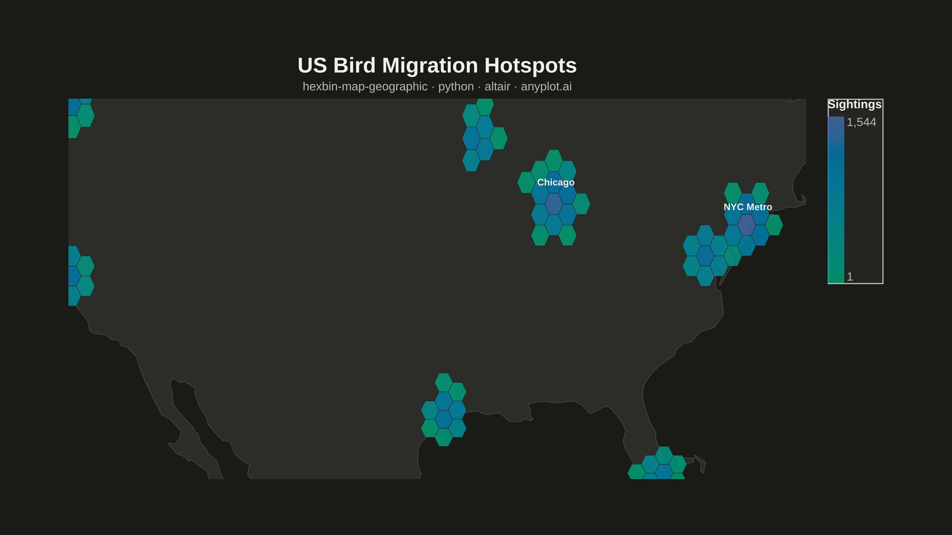
A geographic map visualization that aggregates point data into hexagonal cells, displaying density or aggregated values per cell using color intensity. Unlike continuous heatmaps that use kernel density estimation, hexbin maps provide discrete binning that clearly shows data aggregation boundaries. The hexagonal grid is superior to square grids due to isotropy (equal distance to neighboring cells) and better visual continuity, making it ideal for spatial statistics and urban data analysis.
""" anyplot.ai
hexbin-map-geographic: Hexagonal Binning Map
Library: altair 6.1.0 | Python 3.13.13
Quality: 91/100 | Created: 2026-05-27
"""

import os
import sys
from collections import Counter


# Work around filename shadowing the altair library
sys.path.pop(0)

import altair as alt
import numpy as np
from PIL import Image


# Theme tokens
THEME = os.getenv("ANYPLOT_THEME", "light")
PAGE_BG = "#FAF8F1" if THEME == "light" else "#1A1A17"
ELEVATED_BG = "#FFFDF6" if THEME == "light" else "#242420"
INK = "#1A1A17" if THEME == "light" else "#F0EFE8"
INK_SOFT = "#4A4A44" if THEME == "light" else "#B8B7B0"
LAND_FILL = "#E8E4DC" if THEME == "light" else "#2C2C28"
LAND_STROKE = "#B0AFA8" if THEME == "light" else "#4A4A44"

# Data: bird species sightings — deliberately wide density spread to showcase log-scale range
np.random.seed(42)
# (lat, lon, n_obs, spread_deg) — from sparse (150) to heavy (2500)
clusters = [
    (47.6, -122.3, 2000, 0.45),  # Seattle / Pacific flyway (dense hub)
    (37.8, -122.4, 800, 0.40),  # San Francisco Bay (moderate)
    (29.8, -95.4, 350, 0.40),  # Houston / Gulf Coast (lighter)
    (41.9, -87.6, 1500, 0.45),  # Chicago / Great Lakes (dense hub)
    (40.7, -74.0, 2500, 0.40),  # New York metro (densest hub)
    (38.9, -77.0, 500, 0.38),  # Washington DC (moderate)
    (25.8, -80.2, 150, 0.38),  # Miami / Atlantic flyway (sparse)
    (44.9, -93.2, 250, 0.42),  # Minneapolis / Mississippi corridor (sparse)
]

lats_all, lons_all = [], []
for clat, clon, n, spread in clusters:
    lats_all.extend(np.random.normal(clat, spread, n))
    lons_all.extend(np.random.normal(clon, spread, n))

lats = np.clip(np.array(lats_all), 24.0, 50.0)
lons = np.clip(np.array(lons_all), -126.0, -65.0)

# Flat-top hexagonal binning in lat/lon space
HEX_R = 0.65  # degrees (~65 km at mid-latitudes)
COL_STEP = 1.5 * HEX_R
ROW_STEP = HEX_R * np.sqrt(3)

cols = np.round(lons / COL_STEP).astype(int)
row_off = (np.abs(cols) % 2) * 0.5
rows = np.round(lats / ROW_STEP - row_off).astype(int)
hex_counts = Counter(zip(cols.tolist(), rows.tolist(), strict=False))

features = []
for (c, r), count in hex_counts.items():
    lon_c = c * COL_STEP
    lat_c = (r + (abs(c) % 2) * 0.5) * ROW_STEP
    if not (23.5 <= lat_c <= 51.0 and -127.0 <= lon_c <= -64.0):
        continue
    # Clockwise winding in geographic coords → renders as filled interior
    # (vl-convert flips y-axis; CW geo = CCW screen = D3 interior fill)
    verts = [
        [lon_c + HEX_R * np.cos(np.radians(-60 * i)), lat_c + HEX_R * np.sin(np.radians(-60 * i))] for i in range(6)
    ]
    verts.append(verts[0])
    features.append(
        {
            "type": "Feature",
            "geometry": {"type": "Polygon", "coordinates": [verts]},
            "properties": {"count": int(count)},
        }
    )

# Labels for the three strongest migration hubs — guide viewer to the story
ann_data = [
    {"lon": -74.0, "lat": 41.2, "label": "NYC Metro"},
    {"lon": -122.3, "lat": 47.0, "label": "Seattle"},
    {"lon": -87.6, "lat": 42.5, "label": "Chicago"},
]

# Base map — vega CDN, no local package required
WORLD_URL = "https://cdn.jsdelivr.net/npm/[email protected]/data/world-110m.json"
# Mercator projection centred on continental US, tuned to fit inner 620×320 view
proj_params = {"type": "mercator", "scale": 680, "center": [-96, 37]}

basemap = (
    alt.Chart(alt.topo_feature(WORLD_URL, "land"))
    .mark_geoshape(fill=LAND_FILL, stroke=LAND_STROKE, strokeWidth=0.5)
    .project(**proj_params)
)

# Hexbin layer — inline GeoJSON features, sequential colormap brand-green → blue
hexbin = (
    alt.Chart(alt.InlineData(values=features, format=alt.DataFormat(type="json")))
    .mark_geoshape(stroke=PAGE_BG, strokeWidth=0.3, opacity=0.85)
    .encode(
        color=alt.Color(
            "properties.count:Q",
            scale=alt.Scale(type="log", range=["#009E73", "#4467A3"]),
            legend=alt.Legend(
                title="Sightings", gradientLength=140, gradientThickness=14, labelFontSize=10, titleFontSize=10
            ),
        ),
        tooltip=[alt.Tooltip("properties.count:Q", title="Sightings")],
    )
    .project(**proj_params)
)

# Text annotations directing the viewer to the densest migration hubs
annotation = (
    alt.Chart(alt.InlineData(values=ann_data))
    .mark_text(color=INK, fontSize=8, fontWeight="bold", align="center", dy=-4)
    .encode(longitude="lon:Q", latitude="lat:Q", text="label:N")
    .project(**proj_params)
)

chart = (
    alt.layer(basemap, hexbin, annotation)
    .properties(
        width=620,
        height=320,
        background=PAGE_BG,
        title=alt.TitleParams(
            text="US Bird Migration Hotspots", subtitle="hexbin-map-geographic · python · altair · anyplot.ai"
        ),
        padding={"left": 0, "right": 0, "top": 0, "bottom": 0},
    )
    .configure_title(color=INK, fontSize=18, fontWeight="bold", subtitleColor=INK_SOFT, subtitleFontSize=10)
    .configure_view(fill=PAGE_BG, stroke=None)
    .configure_legend(
        fillColor=ELEVATED_BG,
        strokeColor=INK_SOFT,
        labelColor=INK_SOFT,
        titleColor=INK,
        labelFontSize=10,
        titleFontSize=10,
    )
)

chart.save(f"plot-{THEME}.png", scale_factor=4.0)

TW, TH = 3200, 1800
_img = Image.open(f"plot-{THEME}.png").convert("RGB")
_w, _h = _img.size
if _w > TW or _h > TH:
    raise SystemExit(
        f"altair vl-convert produced {_w}×{_h}, exceeds target {TW}×{TH}. "
        f"Shrink chart .properties(width=, height=) values and re-render."
    )
if _w < TW or _h < TH:
    _canvas = Image.new("RGB", (TW, TH), PAGE_BG)
    _canvas.paste(_img, ((TW - _w) // 2, (TH - _h) // 2))
    _canvas.save(f"plot-{THEME}.png")

chart.save(f"plot-{THEME}.html")
Runnable source as JSON, for any HTTP client: https://api.anyplot.ai/specs/hexbin-map-geographic/altair/code. Any spec id and library id listed in llms-full.txt fit the same URL shape; every URL below is complete and callable.
{
  "spec_id": "hexbin-map-geographic",
  "language": "python",
  "library": "altair",
  "page": "https://anyplot.ai/hexbin-map-geographic/python/altair",
  "hub": "https://anyplot.ai/hexbin-map-geographic",
  "code_json": "https://api.anyplot.ai/specs/hexbin-map-geographic/altair/code",
  "spec_json": "https://api.anyplot.ai/specs/hexbin-map-geographic",
  "render_light_png": "https://storage.googleapis.com/anyplot-images/plots/hexbin-map-geographic/python/altair/plot-light.png",
  "render_dark_png": "https://storage.googleapis.com/anyplot-images/plots/hexbin-map-geographic/python/altair/plot-dark.png",
  "interactive_light_html": "https://storage.googleapis.com/anyplot-images/plots/hexbin-map-geographic/python/altair/plot-light.html",
  "interactive_dark_html": "https://storage.googleapis.com/anyplot-images/plots/hexbin-map-geographic/python/altair/plot-dark.html",
  "quality_score": 91.0,
  "license": "MIT",
  "guide": "https://anyplot.ai/llms.txt"
}
Part of Hexagonal Binning Map on anyplot.ai.