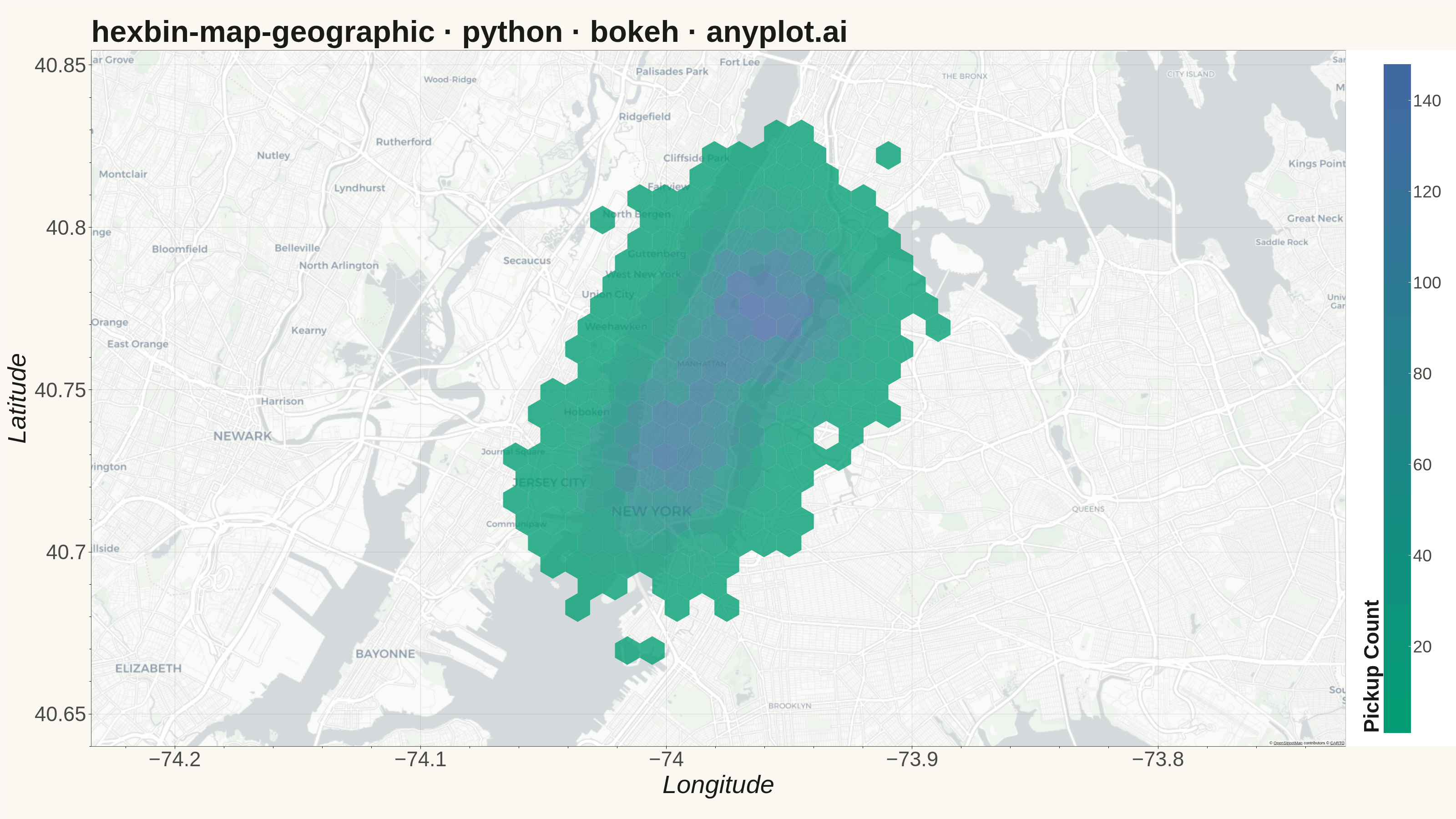
A geographic map visualization that aggregates point data into hexagonal cells, displaying density or aggregated values per cell using color intensity. Unlike continuous heatmaps that use kernel density estimation, hexbin maps provide discrete binning that clearly shows data aggregation boundaries. The hexagonal grid is superior to square grids due to isotropy (equal distance to neighboring cells) and better visual continuity, making it ideal for spatial statistics and urban data analysis.
""" anyplot.ai
hexbin-map-geographic: Hexagonal Binning Map
Library: bokeh 3.9.0 | Python 3.13.13
Quality: 90/100 | Updated: 2026-05-27
"""

import os
import sys


# Remove the script's own directory from sys.path to prevent self-import collision
# (this file is named bokeh.py, which would otherwise shadow the installed bokeh package)
_script_dir = os.path.dirname(os.path.abspath(__file__))
sys.path = [p for p in sys.path if p != "" and os.path.abspath(p) != _script_dir]

import time
from pathlib import Path

import numpy as np
from bokeh.io import output_file, save
from bokeh.models import ColorBar, ColumnDataSource, HoverTool, LinearColorMapper
from bokeh.plotting import figure
from bokeh.transform import transform
from bokeh.util.hex import hexbin
from selenium import webdriver
from selenium.webdriver.chrome.options import Options


# Theme tokens
THEME = os.getenv("ANYPLOT_THEME", "light")
PAGE_BG = "#FAF8F1" if THEME == "light" else "#1A1A17"
ELEVATED_BG = "#FFFDF6" if THEME == "light" else "#242420"
INK = "#1A1A17" if THEME == "light" else "#F0EFE8"
INK_SOFT = "#4A4A44" if THEME == "light" else "#B8B7B0"

# Data — simulated NYC taxi pickup GPS coordinates
np.random.seed(42)
n_points = 8000

cluster_centers = [
    (-73.984, 40.754),  # Times Square / Midtown
    (-73.965, 40.782),  # Upper West Side
    (-74.005, 40.724),  # SoHo / TriBeCa
    (-73.991, 40.735),  # Greenwich Village
    (-73.951, 40.773),  # Carnegie Hill / Museum Mile
]

lon_list = []
lat_list = []
for cx, cy in cluster_centers:
    n = n_points // len(cluster_centers) + np.random.randint(-300, 300)
    lon_list.extend(np.random.normal(cx, 0.018, n))
    lat_list.extend(np.random.normal(cy, 0.014, n))

lon = np.array(lon_list)
lat = np.array(lat_list)

# Web Mercator projection (EPSG:3857)
K = 6378137.0
merc_x = lon * (K * np.pi / 180.0)
merc_y = np.log(np.tan((90.0 + lat) * np.pi / 360.0)) * K

# Hexagonal binning (size in Web Mercator meters)
hex_size = 650
bins = hexbin(merc_x, merc_y, hex_size)
source = ColumnDataSource(data={"q": np.array(bins.q), "r": np.array(bins.r), "counts": np.array(bins.counts)})

# imprint_seq colormap: #009E73 (green) → #4467A3 (blue), 256 stops
c0 = np.array([0x00, 0x9E, 0x73])
c1 = np.array([0x44, 0x67, 0xA3])
t_vals = np.linspace(0, 1, 256)
rgb_ramp = np.round(c0 + np.outer(t_vals, c1 - c0)).astype(int)
imprint_seq = [f"#{r:02X}{g:02X}{b:02X}" for r, g, b in rgb_ramp]

mapper = LinearColorMapper(palette=imprint_seq, low=float(bins.counts.min()), high=float(bins.counts.max()))

# Map viewport with padding
pad = 4000
x_range = (float(merc_x.min()) - pad, float(merc_x.max()) + pad)
y_range = (float(merc_y.min()) - pad, float(merc_y.max()) + pad)

# Title — 51 chars, under 67 baseline, no scaling needed
title = "hexbin-map-geographic · python · bokeh · anyplot.ai"

# Tile layer for geographic context
tile_provider = "CartoDB Dark Matter" if THEME == "dark" else "CartoDB Positron"

# Figure — 3200×1800 landscape, toolbar disabled for exact PNG dimensions
p = figure(
    width=3200,
    height=1800,
    title=title,
    x_axis_label="Longitude",
    y_axis_label="Latitude",
    x_axis_type="mercator",
    y_axis_type="mercator",
    x_range=x_range,
    y_range=y_range,
    toolbar_location=None,
    min_border_bottom=160,
    min_border_left=200,
    min_border_top=110,
    min_border_right=80,
)

# Geographic base layer
p.add_tile(tile_provider)

# Hex tiles
p.hex_tile(
    q="q", r="r", size=hex_size, fill_color=transform("counts", mapper), line_color=None, alpha=0.78, source=source
)

# Hover tooltip
hover = HoverTool(tooltips=[("Taxi Pickups", "@counts"), ("Hex Cell", "(@q, @r)")], mode="mouse")
p.add_tools(hover)

# Color bar
color_bar = ColorBar(
    color_mapper=mapper,
    location=(0, 0),
    title="Pickup Count",
    title_text_font_size="34pt",
    title_text_font_style="bold",
    title_text_color=INK,
    major_label_text_font_size="28pt",
    major_label_text_color=INK_SOFT,
    width=60,
    padding=30,
    margin=40,
)
p.add_layout(color_bar, "right")

# Theme-adaptive chrome
p.background_fill_color = PAGE_BG
p.border_fill_color = PAGE_BG
p.outline_line_color = INK_SOFT

p.title.text_font_size = "50pt"
p.title.text_color = INK
p.title.text_font_style = "bold"

p.xaxis.axis_label_text_font_size = "42pt"
p.yaxis.axis_label_text_font_size = "42pt"
p.xaxis.axis_label_text_color = INK
p.yaxis.axis_label_text_color = INK
p.xaxis.major_label_text_font_size = "34pt"
p.yaxis.major_label_text_font_size = "34pt"
p.xaxis.major_label_text_color = INK_SOFT
p.yaxis.major_label_text_color = INK_SOFT
p.xaxis.axis_line_color = INK_SOFT
p.yaxis.axis_line_color = INK_SOFT
p.xaxis.major_tick_line_color = INK_SOFT
p.yaxis.major_tick_line_color = INK_SOFT

p.xgrid.grid_line_color = INK
p.ygrid.grid_line_color = INK
p.xgrid.grid_line_alpha = 0.12
p.ygrid.grid_line_alpha = 0.12

# Save interactive HTML
output_file(f"plot-{THEME}.html")
save(p)

# Screenshot with headless Chrome — Selenium Manager resolves the driver automatically
W, H = 3200, 1800
opts = Options()
for arg in (
    "--headless=new",
    "--no-sandbox",
    "--disable-dev-shm-usage",
    "--disable-gpu",
    f"--window-size={W},{H}",
    "--hide-scrollbars",
    "--force-device-scale-factor=1",
):
    opts.add_argument(arg)

driver = webdriver.Chrome(options=opts)
driver.set_window_size(W, H)
# Override viewport to exact pixel dimensions (bypasses browser-chrome height overhead)
driver.execute_cdp_cmd(
    "Emulation.setDeviceMetricsOverride", {"width": W, "height": H, "deviceScaleFactor": 1, "mobile": False}
)
driver.get(f"file://{Path(f'plot-{THEME}.html').resolve()}")
time.sleep(5)
driver.save_screenshot(f"plot-{THEME}.png")
driver.quit()
Runnable source as JSON, for any HTTP client: https://api.anyplot.ai/specs/hexbin-map-geographic/bokeh/code. Any spec id and library id listed in llms-full.txt fit the same URL shape; every URL below is complete and callable.
{
  "spec_id": "hexbin-map-geographic",
  "language": "python",
  "library": "bokeh",
  "page": "https://anyplot.ai/hexbin-map-geographic/python/bokeh",
  "hub": "https://anyplot.ai/hexbin-map-geographic",
  "code_json": "https://api.anyplot.ai/specs/hexbin-map-geographic/bokeh/code",
  "spec_json": "https://api.anyplot.ai/specs/hexbin-map-geographic",
  "render_light_png": "https://storage.googleapis.com/anyplot-images/plots/hexbin-map-geographic/python/bokeh/plot-light.png",
  "render_dark_png": "https://storage.googleapis.com/anyplot-images/plots/hexbin-map-geographic/python/bokeh/plot-dark.png",
  "interactive_light_html": "https://storage.googleapis.com/anyplot-images/plots/hexbin-map-geographic/python/bokeh/plot-light.html",
  "interactive_dark_html": "https://storage.googleapis.com/anyplot-images/plots/hexbin-map-geographic/python/bokeh/plot-dark.html",
  "quality_score": 90.0,
  "license": "MIT",
  "guide": "https://anyplot.ai/llms.txt"
}
Part of Hexagonal Binning Map on anyplot.ai.