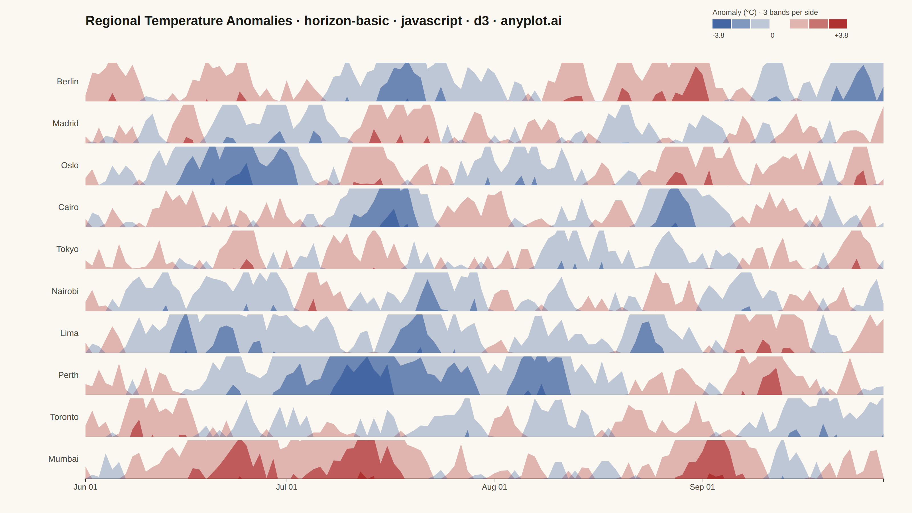
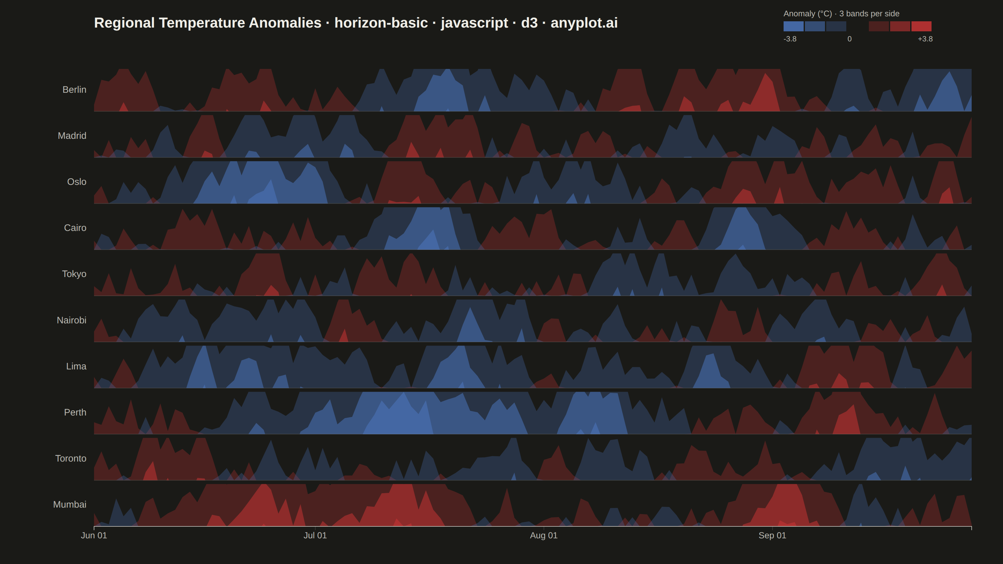
The same plot in 14 other libraries — JavaScript: Chart.js, Apache ECharts, Highcharts, MUI X Charts; Python: Altair, Bokeh, lets-plot, Matplotlib, Plotly, plotnine, Pygal, Seaborn; R: ggplot2; Julia: Makie.jl. Compare all 15 side by side: Horizon Chart in Python, R, Julia and JavaScript.
A horizon chart displays many time series compactly by folding values into color-coded bands, preserving local resolution while minimizing vertical space. It divides the y-axis into bands and uses color intensity to encode magnitude, allowing dozens of series to be compared in limited space. This technique is particularly effective when monitoring many metrics simultaneously where traditional line charts would become unreadable.
// anyplot.ai
// horizon-basic: Horizon Chart
// Library: d3 7.9.0 | JavaScript 22.23.2
// Quality: 92/100 | Created: 2026-08-20

//# anyplot-orientation: landscape
const t = window.ANYPLOT_TOKENS;
const { width, height } = window.ANYPLOT_SIZE;

// --- Data (in-memory, deterministic mean-reverting random walk) ------------
function lcg(seed) {
  let state = seed;
  return function next() {
    state = (state * 1664525 + 1013904223) % 4294967296;
    return state / 4294967296;
  };
}

const stations = [
  "Berlin", "Madrid", "Oslo", "Cairo", "Tokyo",
  "Nairobi", "Lima", "Perth", "Toronto", "Mumbai",
];
const numPoints = 120;
const startDate = new Date(2025, 5, 1);
const dates = Array.from({ length: numPoints }, (_, i) => new Date(startDate.getTime() + i * 86400000));

const series = stations.map((name, si) => {
  const rand = lcg(1000 + si * 37);
  let anomaly = 0;
  const values = dates.map(() => {
    const noise = (rand() - 0.5) * 1.6;
    anomaly = anomaly * 0.9 + noise;
    return anomaly;
  });
  return { name, values };
});

const maxAbs = d3.max(series, (s) => d3.max(s.values, (v) => Math.abs(v)));

// --- SVG mount ---------------------------------------------------------------
const svg = d3.select("#container").append("svg").attr("width", width).attr("height", height);

const margin = { top: 110, right: 50, bottom: 60, left: 150 };
const iw = width - margin.left - margin.right;
const ih = height - margin.top - margin.bottom;

const laneGap = 6;
const laneHeight = (ih - laneGap * (series.length - 1)) / series.length;
const bands = 3;

const x = d3.scaleTime().domain(d3.extent(dates)).range([0, iw]);
// magnitude -> pixel distance folded across `bands` lanes of height laneHeight
const yBand = d3.scaleLinear().domain([0, maxAbs]).range([0, bands * laneHeight]);

// Temperature anomaly is signed/diverging continuous data, so it must use the
// Imprint diverging colormap (t.div = [red, theme-adaptive midpoint, blue]),
// not the categorical palette — and red maps to warm (positive), blue to cold
// (negative), matching the standard NOAA/IPCC temperature-anomaly convention.
const positiveColor = t.div[0]; // "#AE3030" matte red — warm anomaly
const negativeColor = t.div[2]; // "#4467A3" blue — cold anomaly

const root = svg.append("g").attr("transform", `translate(${margin.left},${margin.top})`);

// --- Horizon lanes -----------------------------------------------------------
const areaFor = (accessor) =>
  d3.area()
    .x((d) => x(d.date))
    .y0(laneHeight)
    .y1((d) => laneHeight - yBand(accessor(d)));

series.forEach((s, si) => {
  const rows = dates.map((date, di) => ({ date, value: s.values[di] }));
  const lane = root.append("g").attr("transform", `translate(0,${si * (laneHeight + laneGap)})`);

  lane.append("clipPath")
    .attr("id", `horizon-clip-${si}`)
    .append("rect")
    .attr("width", iw)
    .attr("height", laneHeight);

  // Fold the (band-shifted) path inside a clipped group whose own frame stays
  // fixed to the lane window — the clip must NOT inherit the fold transform,
  // otherwise the visible window would slide along with the data and nothing
  // would ever be cropped into bands.
  const clippedLane = lane.append("g").attr("clip-path", `url(#horizon-clip-${si})`);

  const positiveArea = areaFor((d) => Math.max(d.value, 0));
  const negativeArea = areaFor((d) => Math.max(-d.value, 0));

  for (let i = 0; i < bands; i++) {
    const opacity = (i + 1) / bands;
    clippedLane.append("path")
      .attr("transform", `translate(0,${i * laneHeight})`)
      .datum(rows)
      .attr("d", positiveArea)
      .attr("fill", positiveColor)
      .attr("fill-opacity", opacity);

    clippedLane.append("path")
      .attr("transform", `translate(0,${i * laneHeight})`)
      .datum(rows)
      .attr("d", negativeArea)
      .attr("fill", negativeColor)
      .attr("fill-opacity", opacity);
  }

  lane.append("line")
    .attr("x1", 0).attr("x2", iw)
    .attr("y1", laneHeight).attr("y2", laneHeight)
    .attr("stroke", t.grid).attr("stroke-width", 1);

  lane.append("text")
    .attr("x", -12).attr("y", laneHeight / 2)
    .attr("text-anchor", "end").attr("dominant-baseline", "middle")
    .attr("fill", t.inkSoft).style("font-size", "15px")
    .text(s.name);
});

// --- X axis (below the last lane) --------------------------------------------
const xAxisGroup = root.append("g")
  .attr("transform", `translate(0,${ih})`)
  .call(d3.axisBottom(x).ticks(6).tickFormat(d3.timeFormat("%b %d")));
xAxisGroup.selectAll("text").attr("fill", t.inkSoft).style("font-size", "14px");
xAxisGroup.selectAll("line").attr("stroke", t.grid);
xAxisGroup.select(".domain").attr("stroke", t.inkSoft);

// --- Intensity legend (top-right, explains the color-to-magnitude mapping) ---
const legend = svg.append("g").attr("transform", `translate(${width - margin.right - 300},34)`);
const swatchW = 34;
const swatchH = 16;

legend.append("text")
  .attr("x", 0).attr("y", -8)
  .attr("fill", t.inkSoft).style("font-size", "13px")
  .text(`Anomaly (°C) · ${bands} bands per side`);

for (let i = 0; i < bands; i++) {
  legend.append("rect")
    .attr("x", i * swatchW).attr("y", 0)
    .attr("width", swatchW - 2).attr("height", swatchH)
    .attr("fill", negativeColor).attr("fill-opacity", (bands - i) / bands);
  legend.append("rect")
    .attr("x", (bands + 1 + i) * swatchW).attr("y", 0)
    .attr("width", swatchW - 2).attr("height", swatchH)
    .attr("fill", positiveColor).attr("fill-opacity", (i + 1) / bands);
}
legend.append("text")
  .attr("x", 0).attr("y", swatchH + 16)
  .attr("fill", t.inkSoft).style("font-size", "12px")
  .text(`-${maxAbs.toFixed(1)}`);
legend.append("text")
  .attr("x", bands * swatchW).attr("y", swatchH + 16)
  .attr("fill", t.inkSoft).style("font-size", "12px")
  .text("0");
legend.append("text")
  .attr("x", (2 * bands + 1) * swatchW).attr("y", swatchH + 16)
  .attr("text-anchor", "end")
  .attr("fill", t.inkSoft).style("font-size", "12px")
  .text(`+${maxAbs.toFixed(1)}`);

// --- Title ---------------------------------------------------------------------
// Title fontsize scales linearly off the 67-char mandated-title baseline
// (default 26px @ 67 chars) so the descriptive prefix never overflows while
// still filling a healthy share of the plot width.
const titleText = "Regional Temperature Anomalies · horizon-basic · javascript · d3 · anyplot.ai";
const titleFontSize = Math.round(26 * Math.min(1, 67 / titleText.length));
svg.append("text")
  .attr("x", margin.left).attr("y", 44)
  .attr("fill", t.ink).style("font-size", `${titleFontSize}px`).style("font-weight", "600")
  .text(titleText);
Runnable source as JSON, for any HTTP client: https://api.anyplot.ai/specs/horizon-basic/d3/code. Any spec id and library id listed in llms-full.txt fit the same URL shape; every URL below is complete and callable.
{
  "spec_id": "horizon-basic",
  "language": "javascript",
  "library": "d3",
  "page": "https://anyplot.ai/horizon-basic/javascript/d3",
  "hub": "https://anyplot.ai/horizon-basic",
  "code_json": "https://api.anyplot.ai/specs/horizon-basic/d3/code",
  "spec_json": "https://api.anyplot.ai/specs/horizon-basic",
  "render_light_png": "https://storage.googleapis.com/anyplot-images/plots/horizon-basic/javascript/d3/plot-light.png",
  "render_dark_png": "https://storage.googleapis.com/anyplot-images/plots/horizon-basic/javascript/d3/plot-dark.png",
  "interactive_light_html": "https://storage.googleapis.com/anyplot-images/plots/horizon-basic/javascript/d3/plot-light.html",
  "interactive_dark_html": "https://storage.googleapis.com/anyplot-images/plots/horizon-basic/javascript/d3/plot-dark.html",
  "quality_score": 92.0,
  "license": "MIT",
  "guide": "https://anyplot.ai/llms.txt"
}
Part of Horizon Chart on anyplot.ai.