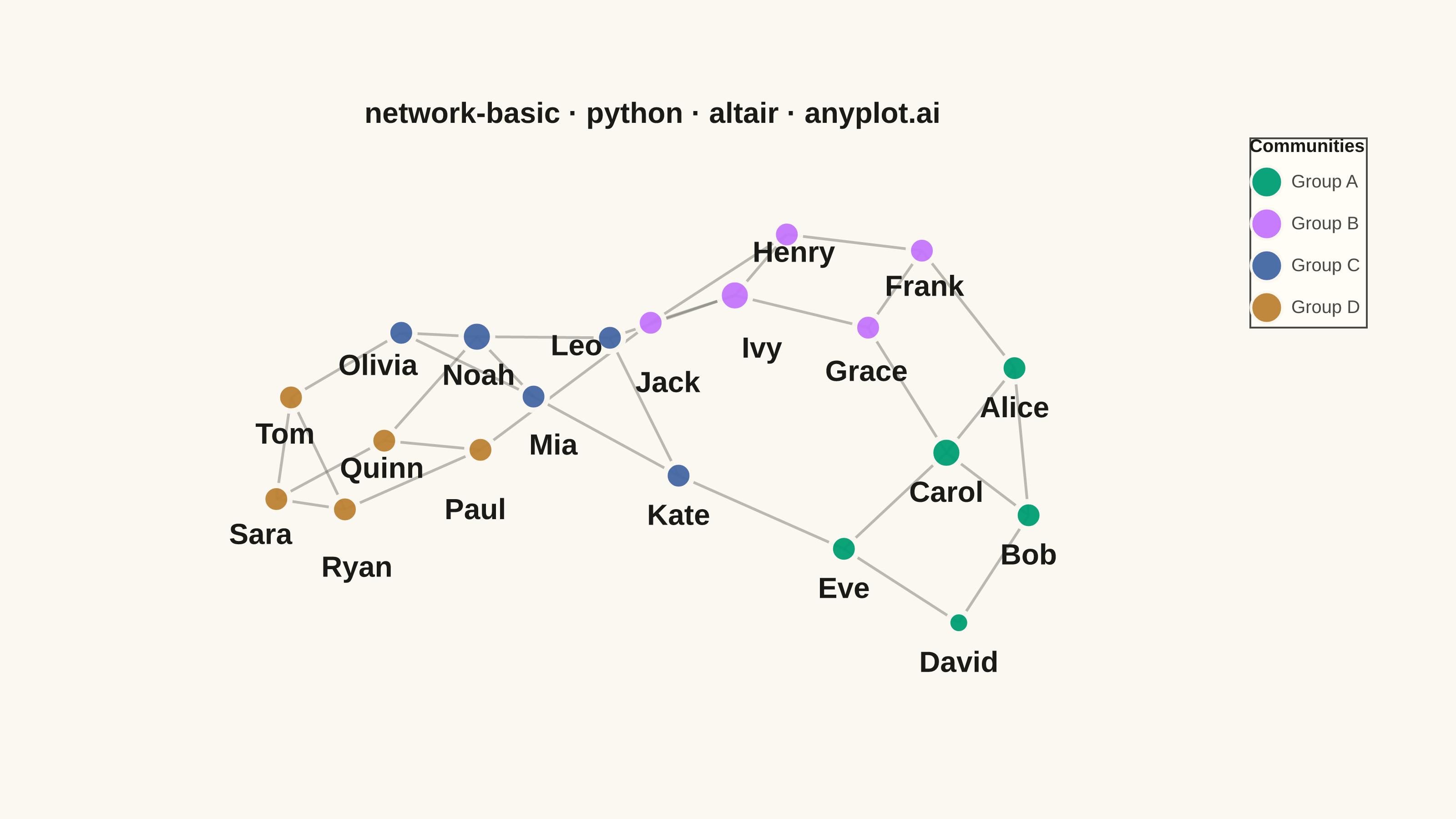
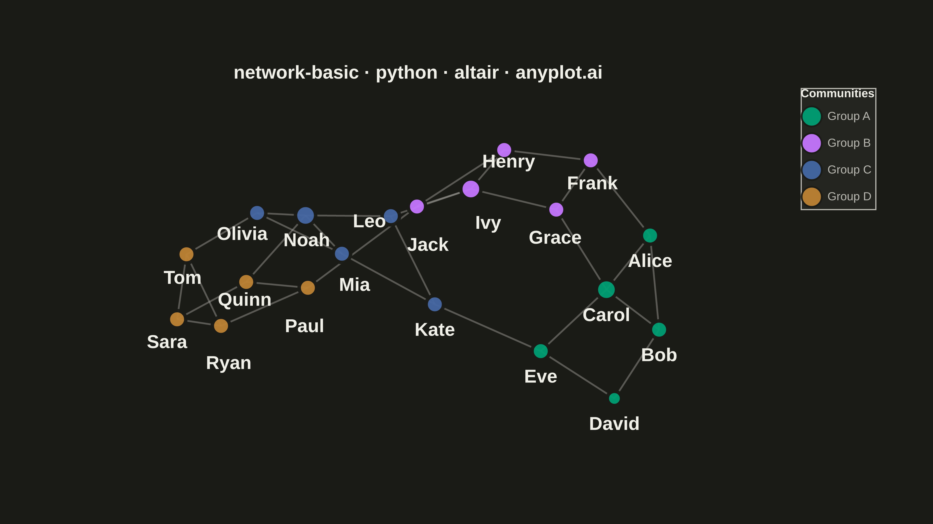
A network graph (node-link diagram) visualizes relationships between entities as nodes connected by edges. It reveals the structure of connections, clusters, and central nodes in relational data. Network graphs are essential for understanding complex systems where relationships matter as much as the entities themselves, making hidden patterns of connectivity visible at a glance.
""" anyplot.ai
network-basic: Basic Network Graph
Library: altair 6.2.2 | Python 3.13.14
Quality: 87/100 | Updated: 2026-07-24
"""

import os

import altair as alt
import numpy as np
import pandas as pd
from PIL import Image


# Theme-adaptive chrome tokens
THEME = os.getenv("ANYPLOT_THEME", "light")
PAGE_BG = "#FAF8F1" if THEME == "light" else "#1A1A17"
ELEVATED_BG = "#FFFDF6" if THEME == "light" else "#242420"
INK = "#1A1A17" if THEME == "light" else "#F0EFE8"
INK_SOFT = "#4A4A44" if THEME == "light" else "#B8B7B0"
INK_MUTED = "#6B6A63" if THEME == "light" else "#A8A79F"

# Imprint categorical palette (first 4 slots, canonical order — groups are abstract)
IMPRINT_PALETTE = ["#009E73", "#C475FD", "#4467A3", "#BD8233", "#AE3030", "#2ABCCD", "#954477", "#99B314"]

# Set seed for reproducibility
np.random.seed(42)

# Data: A small social network with 20 people in 4 communities
nodes = [
    {"id": 0, "label": "Alice", "group": "Group A"},
    {"id": 1, "label": "Bob", "group": "Group A"},
    {"id": 2, "label": "Carol", "group": "Group A"},
    {"id": 3, "label": "David", "group": "Group A"},
    {"id": 4, "label": "Eve", "group": "Group A"},
    {"id": 5, "label": "Frank", "group": "Group B"},
    {"id": 6, "label": "Grace", "group": "Group B"},
    {"id": 7, "label": "Henry", "group": "Group B"},
    {"id": 8, "label": "Ivy", "group": "Group B"},
    {"id": 9, "label": "Jack", "group": "Group B"},
    {"id": 10, "label": "Kate", "group": "Group C"},
    {"id": 11, "label": "Leo", "group": "Group C"},
    {"id": 12, "label": "Mia", "group": "Group C"},
    {"id": 13, "label": "Noah", "group": "Group C"},
    {"id": 14, "label": "Olivia", "group": "Group C"},
    {"id": 15, "label": "Paul", "group": "Group D"},
    {"id": 16, "label": "Quinn", "group": "Group D"},
    {"id": 17, "label": "Ryan", "group": "Group D"},
    {"id": 18, "label": "Sara", "group": "Group D"},
    {"id": 19, "label": "Tom", "group": "Group D"},
]

# Edges: Friendship connections (within and between groups)
edges = [
    # Group A internal connections
    (0, 1),
    (0, 2),
    (1, 2),
    (1, 3),
    (2, 4),
    (3, 4),
    # Group B internal connections
    (5, 6),
    (5, 7),
    (6, 8),
    (7, 8),
    (7, 9),
    (8, 9),
    # Group C internal connections
    (10, 11),
    (10, 12),
    (11, 13),
    (12, 13),
    (12, 14),
    (13, 14),
    # Group D internal connections
    (15, 16),
    (15, 17),
    (16, 18),
    (17, 18),
    (17, 19),
    (18, 19),
    # Cross-group connections (bridges between communities)
    (0, 5),
    (4, 10),
    (9, 15),
    (14, 19),
    (2, 6),
    (8, 11),
    (13, 16),
]

# Calculate spring layout (force-directed algorithm)
n = len(nodes)
positions = np.random.rand(n, 2) * 2 - 1
k = 0.4  # Optimal distance parameter

for iteration in range(150):
    displacement = np.zeros((n, 2))

    # Repulsive forces between all node pairs
    for i in range(n):
        for j in range(i + 1, n):
            diff = positions[i] - positions[j]
            dist = max(np.linalg.norm(diff), 0.01)
            force = (k * k / dist) * (diff / dist)
            displacement[i] += force
            displacement[j] -= force

    # Attractive forces for edges
    for src, tgt in edges:
        diff = positions[src] - positions[tgt]
        dist = max(np.linalg.norm(diff), 0.01)
        force = (dist * dist / k) * (diff / dist)
        displacement[src] -= force
        displacement[tgt] += force

    # Apply displacement with cooling
    cooling = 1 - iteration / 150
    for i in range(n):
        disp_norm = np.linalg.norm(displacement[i])
        if disp_norm > 0:
            positions[i] += (displacement[i] / disp_norm) * min(disp_norm, 0.1 * cooling)

# Rotate positions so the network's principal axis aligns with the wide (x)
# canvas dimension. The spring layout otherwise tends to settle into a
# diagonal band, which — even after per-axis normalization — leaves large
# empty triangular regions in two corners of the landscape canvas.
centered = positions - positions.mean(axis=0)
cov = np.cov(centered.T)
eigvals, eigvecs = np.linalg.eigh(cov)
principal = eigvecs[:, np.argmax(eigvals)]
angle = np.arctan2(principal[1], principal[0])
rotation = np.array([[np.cos(-angle), -np.sin(-angle)], [np.sin(-angle), np.cos(-angle)]])
positions = centered @ rotation.T

# Normalize positions to [0.1, 0.9] range
pos_min = positions.min(axis=0)
pos_max = positions.max(axis=0)
positions = (positions - pos_min) / (pos_max - pos_min + 1e-6) * 0.8 + 0.1
pos = {node["id"]: positions[i] for i, node in enumerate(nodes)}

# Calculate node degrees for sizing
degrees = {node["id"]: 0 for node in nodes}
for src, tgt in edges:
    degrees[src] += 1
    degrees[tgt] += 1

# Anti-collision label layout: start each label just below its node, in
# pixel space (the 620x320 view is much wider than tall, so a fixed offset
# in data units isn't visually isotropic), then run a short repulsion pass
# so labels that would otherwise collide (Jack/Leo, Noah/Olivia, the
# Quinn/Ryan/Sara chain, ...) push apart from each other in both x and y
# instead of overlapping. A spring-back pull toward each label's own base
# offset (plus a hard clamp on drift distance) keeps every label anchored
# close to its own node, so it never reads as ambiguous or lands on top of
# a neighboring marker.
coords = np.array([pos[node["id"]] for node in nodes])
VIEW_W, VIEW_H, DOMAIN_SPAN = 620, 320, 1.1
px_per_x, px_per_y = VIEW_W / DOMAIN_SPAN, VIEW_H / DOMAIN_SPAN
node_px = coords * np.array([px_per_x, px_per_y])
base_px_offset = np.tile(np.array([0.0, -24.0]), (n, 1))
label_px_offset = base_px_offset.copy()
min_label_dist_px = 62.0
max_drift_px = 46.0
for _ in range(60):
    label_px = node_px + label_px_offset
    disp = np.zeros((n, 2))
    for i in range(n):
        for j in range(i + 1, n):
            diff = label_px[i] - label_px[j]
            dist = max(np.linalg.norm(diff), 0.5)
            if dist < min_label_dist_px:
                push = (min_label_dist_px - dist) * 0.5 * (diff / dist)
                disp[i] += push
                disp[j] -= push
    label_px_offset += disp
    label_px_offset += (base_px_offset - label_px_offset) * 0.05
    drift_norm = np.linalg.norm(label_px_offset, axis=1, keepdims=True)
    too_far = drift_norm[:, 0] > max_drift_px
    if too_far.any():
        label_px_offset[too_far] = label_px_offset[too_far] / drift_norm[too_far] * max_drift_px
label_offset = label_px_offset / np.array([px_per_x, px_per_y])
label_dx = label_offset[:, 0]
label_dy = label_offset[:, 1]

# Create nodes dataframe. label_x/label_y carry the anti-collision offset.
nodes_df = pd.DataFrame(
    [
        {
            "id": node["id"],
            "label": node["label"],
            "group": node["group"],
            "x": pos[node["id"]][0],
            "y": pos[node["id"]][1],
            "label_x": pos[node["id"]][0] + label_dx[i],
            "label_y": pos[node["id"]][1] + label_dy[i],
            "degree": degrees[node["id"]],
        }
        for i, node in enumerate(nodes)
    ]
)

# Create edges dataframe with coordinates for each edge segment
edges_df = pd.DataFrame(
    [{"edge_id": i, "x": pos[src][0], "y": pos[src][1], "order": 0} for i, (src, _) in enumerate(edges)]
    + [{"edge_id": i, "x": pos[tgt][0], "y": pos[tgt][1], "order": 1} for i, (_, tgt) in enumerate(edges)]
)

# Draw edges as lines (muted, theme-adaptive — structural, not data-categorical)
edges_chart = (
    alt.Chart(edges_df)
    .mark_line(strokeWidth=1.5, opacity=0.45, color=INK_MUTED)
    .encode(
        x=alt.X("x:Q", scale=alt.Scale(domain=[-0.05, 1.05]), axis=None),
        y=alt.Y("y:Q", scale=alt.Scale(domain=[-0.05, 1.05]), axis=None),
        detail="edge_id:N",
        order="order:O",
    )
)

# Draw nodes as points (size based on degree; PAGE_BG stroke halos each node
# against overlapping edges/labels and stays correct in both themes)
nodes_chart = (
    alt.Chart(nodes_df)
    .mark_circle(stroke=PAGE_BG, strokeWidth=3, opacity=0.95)
    .encode(
        x=alt.X("x:Q", scale=alt.Scale(domain=[-0.05, 1.05]), axis=None),
        y=alt.Y("y:Q", scale=alt.Scale(domain=[-0.05, 1.05]), axis=None),
        size=alt.Size("degree:Q", scale=alt.Scale(domain=[2, 6], range=[150, 450]), legend=None),
        color=alt.Color(
            "group:N",
            scale=alt.Scale(domain=["Group A", "Group B", "Group C", "Group D"], range=IMPRINT_PALETTE[:4]),
            legend=alt.Legend(title="Communities", symbolSize=300),
        ),
        tooltip=["label:N", "group:N", "degree:Q"],
    )
)

# Draw node labels (label_x/label_y already carry the anti-collision offset)
labels_chart = (
    alt.Chart(nodes_df)
    .mark_text(fontSize=16, fontWeight="bold", color=INK)
    .encode(x=alt.X("label_x:Q"), y=alt.Y("label_y:Q"), text="label:N")
)

# Combine layers with theme-adaptive chrome
chart = (
    (edges_chart + nodes_chart + labels_chart)
    .properties(
        width=620,  # inner-view — see prompts/library/altair.md "Canvas — hard rule"
        height=320,
        background=PAGE_BG,
        title=alt.Title("network-basic · python · altair · anyplot.ai", fontSize=16),
    )
    .configure_view(fill=PAGE_BG, stroke=None, continuousWidth=620, continuousHeight=320)
    .configure_title(color=INK)
    .configure_legend(
        fillColor=ELEVATED_BG,
        strokeColor=INK_SOFT,
        labelColor=INK_SOFT,
        titleColor=INK,
        labelFontSize=10,
        titleFontSize=10,
    )
)

# Save as PNG and HTML
chart.save(f"plot-{THEME}.png", scale_factor=4.0)
chart.save(f"plot-{THEME}.html")

# Pad the saved PNG up to the exact canonical target (3200x1800). Never crop —
# cropping would clip title/legend text at the edges. See "Canvas" in
# prompts/library/altair.md.
TW, TH = 3200, 1800
_img = Image.open(f"plot-{THEME}.png").convert("RGB")
_w, _h = _img.size
if _w > TW or _h > TH:
    raise SystemExit(
        f"altair vl-convert produced {_w}x{_h}, exceeds target {TW}x{TH}. "
        f"Shrink chart .properties(width=, height=) values and re-render."
    )
if _w < TW or _h < TH:
    _canvas = Image.new("RGB", (TW, TH), PAGE_BG)
    _canvas.paste(_img, ((TW - _w) // 2, (TH - _h) // 2))
    _canvas.save(f"plot-{THEME}.png")
Runnable source as JSON, for any HTTP client: https://api.anyplot.ai/specs/network-basic/altair/code. Any spec id and library id listed in llms-full.txt fit the same URL shape; every URL below is complete and callable.
{
  "spec_id": "network-basic",
  "language": "python",
  "library": "altair",
  "page": "https://anyplot.ai/network-basic/python/altair",
  "hub": "https://anyplot.ai/network-basic",
  "code_json": "https://api.anyplot.ai/specs/network-basic/altair/code",
  "spec_json": "https://api.anyplot.ai/specs/network-basic",
  "render_light_png": "https://storage.googleapis.com/anyplot-images/plots/network-basic/python/altair/plot-light.png",
  "render_dark_png": "https://storage.googleapis.com/anyplot-images/plots/network-basic/python/altair/plot-dark.png",
  "interactive_light_html": "https://storage.googleapis.com/anyplot-images/plots/network-basic/python/altair/plot-light.html",
  "interactive_dark_html": "https://storage.googleapis.com/anyplot-images/plots/network-basic/python/altair/plot-dark.html",
  "quality_score": 87.0,
  "license": "MIT",
  "guide": "https://anyplot.ai/llms.txt"
}
Part of Basic Network Graph on anyplot.ai.