The same plot in 14 other libraries — Python: Altair, Bokeh, lets-plot, Matplotlib, Plotly, plotnine, Pygal, Seaborn; Julia: Makie.jl; JavaScript: Chart.js, D3.js, Apache ECharts, Highcharts, MUI X Charts. Compare all 15 side by side: Basic Network Graph in Python, R, Julia and JavaScript.
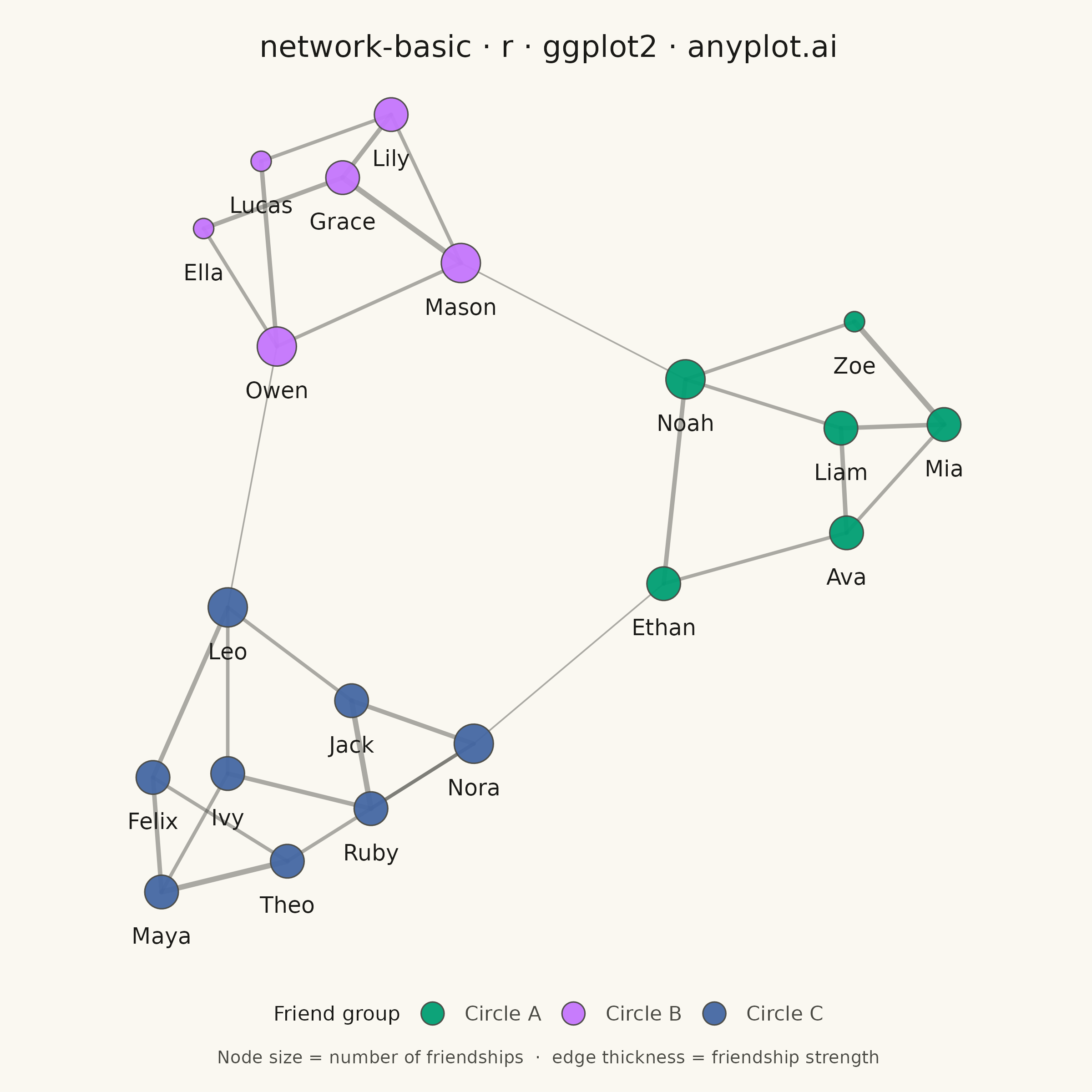
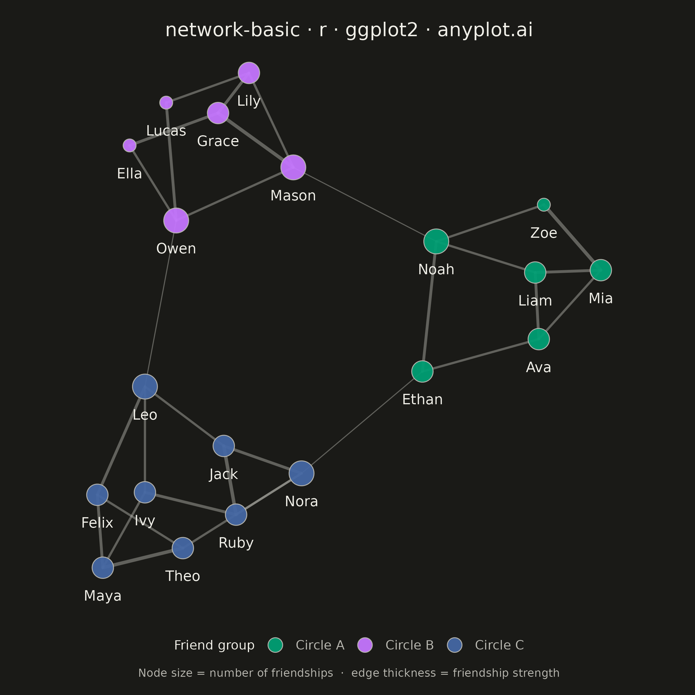
A network graph (node-link diagram) visualizes relationships between entities as nodes connected by edges. It reveals the structure of connections, clusters, and central nodes in relational data. Network graphs are essential for understanding complex systems where relationships matter as much as the entities themselves, making hidden patterns of connectivity visible at a glance.
#' anyplot.ai
#' network-basic: Basic Network Graph
#' Library: ggplot2 3.5.1 | R 4.4.1
#' Quality: 87/100 | Created: 2026-07-24

library(ggplot2)
library(dplyr)
library(ragg)

set.seed(42)

# --- Theme tokens -------------------------------------------------------
THEME    <- Sys.getenv("ANYPLOT_THEME", "light")
PAGE_BG  <- if (THEME == "light") "#FAF8F1" else "#1A1A17"
INK      <- if (THEME == "light") "#1A1A17" else "#F0EFE8"
INK_SOFT <- if (THEME == "light") "#4A4A44" else "#B8B7B0"
IMPRINT_PALETTE <- c("#009E73", "#C475FD", "#4467A3", "#BD8233",
                     "#AE3030", "#2ABCCD", "#954477", "#99B314")

# --- Data: friendship network across three social circles ---------------
names <- c(
  "Ava", "Liam", "Mia", "Noah", "Zoe", "Ethan",
  "Lily", "Mason", "Grace", "Owen", "Ella", "Lucas",
  "Nora", "Jack", "Ruby", "Leo", "Ivy", "Felix", "Maya", "Theo"
)
# Each id belongs to one of three friend circles; a handful of cross-circle
# edges below bridge them, matching the spec's "identify communities" use case.
group <- c(rep("Circle A", 6), rep("Circle B", 6), rep("Circle C", 8))
nodes <- tibble::tibble(id = seq_along(names), name = names, group = group)

edges <- tibble::tibble(
  from = c(1, 1, 2, 2, 3, 4, 4, 1,
           7, 7, 8, 8, 9, 10, 10, 7,
           13, 13, 14, 14, 15, 16, 16, 17, 18, 18, 19, 13,
           4, 6, 10),
  to   = c(2, 3, 3, 4, 5, 5, 6, 6,
           8, 9, 9, 10, 11, 11, 12, 12,
           14, 15, 15, 16, 17, 17, 18, 19, 19, 20, 20, 20,
           8, 13, 16),
  # Friendship strength: within-circle ties run stronger than the sparse
  # cross-circle bridges (last 3 edges), giving edges a second data dimension.
  weight = c(4, 3, 4, 3, 5, 3, 4, 3,
             3, 4, 5, 3, 4, 3, 4, 3,
             4, 3, 5, 3, 4, 3, 4, 3, 4, 3, 5, 3,
             1, 1, 1)
)

n_nodes <- nrow(nodes)
edge_i  <- edges$from
edge_j  <- edges$to

# --- Force-directed layout (Fruchterman-Reingold) ------------------------
# Positions start random, then repulsion (all pairs) and attraction (edges)
# iterate under a cooling schedule until the network settles into a
# readable, cluster-revealing arrangement. No layout package required.
area <- 4
k    <- sqrt(area / n_nodes)
temp <- 0.15
iterations <- 300

pos <- tibble::tibble(x = runif(n_nodes, -1, 1), y = runif(n_nodes, -1, 1))

for (iter in seq_len(iterations)) {
  dx <- outer(pos$x, pos$x, "-")
  dy <- outer(pos$y, pos$y, "-")
  dist_mat <- sqrt(dx^2 + dy^2)
  diag(dist_mat) <- 1

  rep_force <- (k^2) / dist_mat
  fx <- rowSums(rep_force * dx / dist_mat)
  fy <- rowSums(rep_force * dy / dist_mat)

  edx <- pos$x[edge_i] - pos$x[edge_j]
  edy <- pos$y[edge_i] - pos$y[edge_j]
  edist <- pmax(sqrt(edx^2 + edy^2), 0.01)
  att_force <- (edist^2) / k
  fax <- att_force * edx / edist
  fay <- att_force * edy / edist

  for (e in seq_along(edge_i)) {
    fx[edge_i[e]] <- fx[edge_i[e]] - fax[e]
    fy[edge_i[e]] <- fy[edge_i[e]] - fay[e]
    fx[edge_j[e]] <- fx[edge_j[e]] + fax[e]
    fy[edge_j[e]] <- fy[edge_j[e]] + fay[e]
  }

  disp <- pmax(sqrt(fx^2 + fy^2), 0.01)
  step <- pmin(disp, temp)
  pos$x <- pos$x + (fx / disp) * step
  pos$y <- pos$y + (fy / disp) * step

  temp <- temp * 0.99
}

# Rescale to a fixed coordinate span so text nudges/sizes stay predictable
span <- max(abs(c(pos$x, pos$y)))
nodes$x <- pos$x / span * 5
nodes$y <- pos$y / span * 5

# Degree = number of connections per node (drives node size)
degree <- tabulate(c(edge_i, edge_j), nbins = n_nodes)
nodes$degree <- degree

edges_pos <- edges %>%
  left_join(nodes %>% select(id, x, y), by = c("from" = "id")) %>%
  rename(x_from = x, y_from = y) %>%
  left_join(nodes %>% select(id, x, y), by = c("to" = "id")) %>%
  rename(x_to = x, y_to = y)

# --- Plot -----------------------------------------------------------------
anyplot_theme <- theme_minimal(base_size = 8) +
  theme(
    plot.background   = element_rect(fill = PAGE_BG, color = PAGE_BG),
    panel.background  = element_rect(fill = PAGE_BG, color = NA),
    panel.grid        = element_blank(),
    axis.title        = element_blank(),
    axis.text         = element_blank(),
    axis.ticks        = element_blank(),
    legend.position   = "bottom",
    legend.title      = element_text(color = INK, size = 8),
    legend.text       = element_text(color = INK_SOFT, size = 8),
    legend.key        = element_rect(fill = PAGE_BG, color = NA),
    legend.background = element_rect(fill = PAGE_BG, color = NA),
    legend.margin     = margin(t = -4),
    plot.title        = element_text(color = INK, size = 12, hjust = 0.5),
    plot.caption      = element_text(color = INK_SOFT, size = 7, hjust = 0.5, margin = margin(t = 6)),
    plot.margin       = margin(14, 14, 10, 14, "pt")
  )

p <- ggplot() +
  geom_segment(
    data = edges_pos,
    aes(x = x_from, y = y_from, xend = x_to, yend = y_to, linewidth = weight),
    color = INK_SOFT, alpha = 0.45, lineend = "round"
  ) +
  geom_point(
    data = nodes,
    aes(x = x, y = y, size = degree, fill = group),
    shape = 21, color = INK_SOFT, stroke = 0.4, alpha = 0.95
  ) +
  geom_text(
    data = nodes,
    aes(x = x, y = y, label = name),
    color = INK, size = 3.1, nudge_y = -0.42
  ) +
  scale_size(range = c(3.5, 7), guide = "none") +
  scale_linewidth(range = c(0.3, 1.0), guide = "none") +
  scale_fill_manual(values = IMPRINT_PALETTE[1:3], name = "Friend group") +
  coord_equal(clip = "off") +
  labs(
    title   = "network-basic · r · ggplot2 · anyplot.ai",
    caption = "Node size = number of friendships  ·  edge thickness = friendship strength"
  ) +
  guides(fill = guide_legend(override.aes = list(size = 4))) +
  anyplot_theme

# --- Save -------------------------------------------------------------------
ggsave(
  filename = sprintf("plot-%s.png", THEME),
  plot     = p,
  device   = ragg::agg_png,
  width    = 6,
  height   = 6,
  units    = "in",
  dpi      = 400
)
Runnable source as JSON, for any HTTP client: https://api.anyplot.ai/specs/network-basic/ggplot2/code. Any spec id and library id listed in llms-full.txt fit the same URL shape; every URL below is complete and callable.
{
  "spec_id": "network-basic",
  "language": "r",
  "library": "ggplot2",
  "page": "https://anyplot.ai/network-basic/r/ggplot2",
  "hub": "https://anyplot.ai/network-basic",
  "code_json": "https://api.anyplot.ai/specs/network-basic/ggplot2/code",
  "spec_json": "https://api.anyplot.ai/specs/network-basic",
  "render_light_png": "https://storage.googleapis.com/anyplot-images/plots/network-basic/r/ggplot2/plot-light.png",
  "render_dark_png": "https://storage.googleapis.com/anyplot-images/plots/network-basic/r/ggplot2/plot-dark.png",
  "quality_score": 87.0,
  "license": "MIT",
  "guide": "https://anyplot.ai/llms.txt"
}
Part of Basic Network Graph on anyplot.ai.