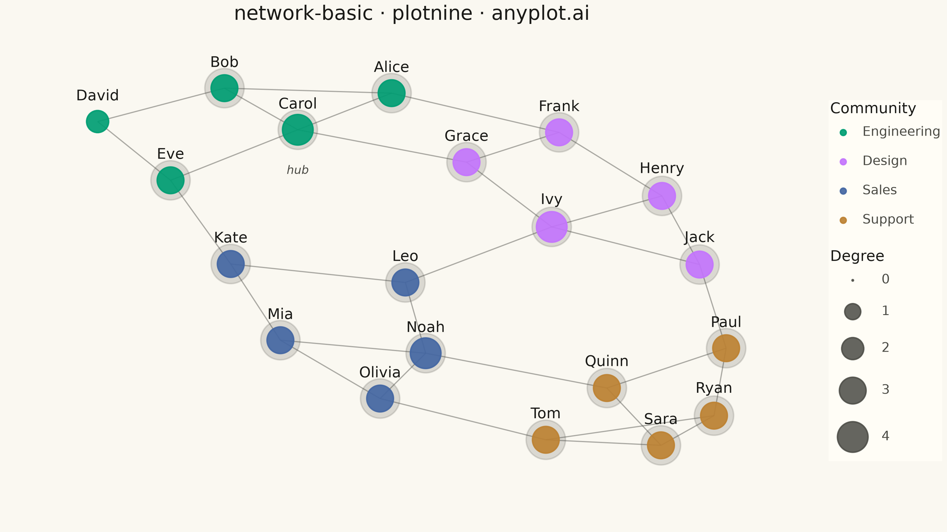
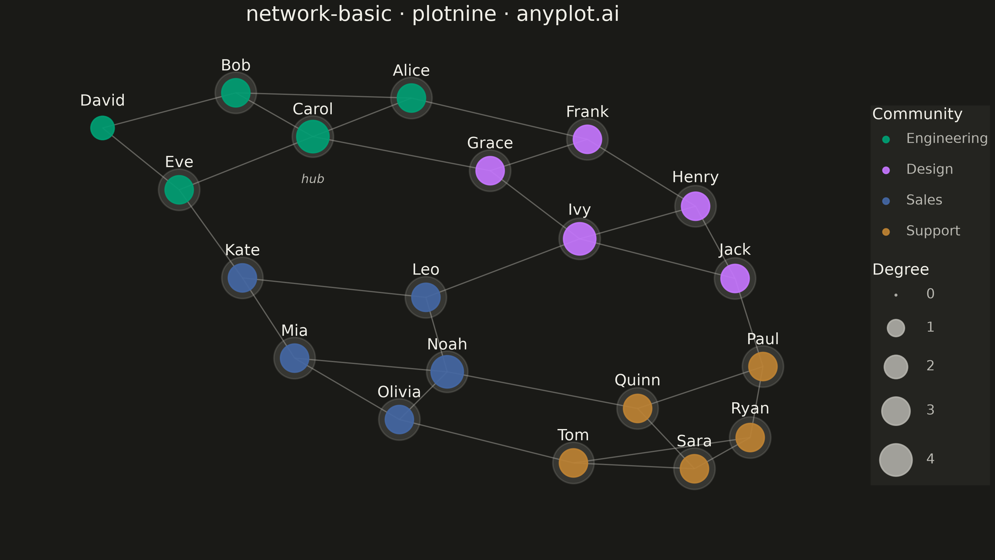
A network graph (node-link diagram) visualizes relationships between entities as nodes connected by edges. It reveals the structure of connections, clusters, and central nodes in relational data. Network graphs are essential for understanding complex systems where relationships matter as much as the entities themselves, making hidden patterns of connectivity visible at a glance.
""" anyplot.ai
network-basic: Basic Network Graph
Library: plotnine 0.15.7 | Python 3.13.14
Quality: 89/100 | Updated: 2026-07-24
"""

import os
import sys

import numpy as np
import pandas as pd


try:
    from plotnine import (
        aes,
        annotate,
        coord_cartesian,
        element_blank,
        element_rect,
        element_text,
        geom_point,
        geom_segment,
        geom_text,
        ggplot,
        guide_legend,
        labs,
        scale_color_manual,
        scale_size_area,
        theme,
    )
except ImportError:
    # This file is named plotnine.py; remove current dir so the library is found instead
    sys.path = [p for p in sys.path if os.path.abspath(p) != os.path.dirname(os.path.abspath(__file__))]
    from plotnine import (
        aes,
        annotate,
        coord_cartesian,
        element_blank,
        element_rect,
        element_text,
        geom_point,
        geom_segment,
        geom_text,
        ggplot,
        guide_legend,
        labs,
        scale_color_manual,
        scale_size_area,
        theme,
    )


# Theme tokens
THEME = os.getenv("ANYPLOT_THEME", "light")
PAGE_BG = "#FAF8F1" if THEME == "light" else "#1A1A17"
ELEVATED_BG = "#FFFDF6" if THEME == "light" else "#242420"
INK = "#1A1A17" if THEME == "light" else "#F0EFE8"
INK_SOFT = "#4A4A44" if THEME == "light" else "#B8B7B0"

IMPRINT = ["#009E73", "#C475FD", "#4467A3", "#BD8233"]

# Data: social network with 20 people in 4 communities
np.random.seed(42)

nodes = [
    {"id": 0, "label": "Alice", "group": "Engineering"},
    {"id": 1, "label": "Bob", "group": "Engineering"},
    {"id": 2, "label": "Carol", "group": "Engineering"},
    {"id": 3, "label": "David", "group": "Engineering"},
    {"id": 4, "label": "Eve", "group": "Engineering"},
    {"id": 5, "label": "Frank", "group": "Design"},
    {"id": 6, "label": "Grace", "group": "Design"},
    {"id": 7, "label": "Henry", "group": "Design"},
    {"id": 8, "label": "Ivy", "group": "Design"},
    {"id": 9, "label": "Jack", "group": "Design"},
    {"id": 10, "label": "Kate", "group": "Sales"},
    {"id": 11, "label": "Leo", "group": "Sales"},
    {"id": 12, "label": "Mia", "group": "Sales"},
    {"id": 13, "label": "Noah", "group": "Sales"},
    {"id": 14, "label": "Olivia", "group": "Sales"},
    {"id": 15, "label": "Paul", "group": "Support"},
    {"id": 16, "label": "Quinn", "group": "Support"},
    {"id": 17, "label": "Ryan", "group": "Support"},
    {"id": 18, "label": "Sara", "group": "Support"},
    {"id": 19, "label": "Tom", "group": "Support"},
]

edges = [
    (0, 1),
    (0, 2),
    (1, 2),
    (1, 3),
    (2, 4),
    (3, 4),
    (5, 6),
    (5, 7),
    (6, 8),
    (7, 8),
    (7, 9),
    (8, 9),
    (10, 11),
    (10, 12),
    (11, 13),
    (12, 13),
    (12, 14),
    (13, 14),
    (15, 16),
    (15, 17),
    (16, 18),
    (17, 18),
    (17, 19),
    (18, 19),
    (0, 5),
    (4, 10),
    (9, 15),
    (14, 19),
    (2, 6),
    (8, 11),
    (13, 16),
]

# Node degrees
n = len(nodes)
degrees = {node["id"]: 0 for node in nodes}
for src, tgt in edges:
    degrees[src] += 1
    degrees[tgt] += 1

# Quadrant-based initialization for balanced 4-cluster arrangement
quadrant_centers = {
    "Engineering": np.array([-0.6, 0.6]),
    "Design": np.array([0.6, 0.6]),
    "Sales": np.array([-0.6, -0.6]),
    "Support": np.array([0.6, -0.6]),
}
positions = np.zeros((n, 2))
for i, node in enumerate(nodes):
    positions[i] = quadrant_centers[node["group"]] + np.random.randn(2) * 0.12

# Vectorized Fruchterman-Reingold spring layout
k = 0.52
for iteration in range(200):
    diff = positions[:, None, :] - positions[None, :, :]  # (n, n, 2)
    dist = np.linalg.norm(diff, axis=2, keepdims=True).clip(0.01)
    repulsion = (k * k / dist**2) * diff
    np.fill_diagonal(repulsion[:, :, 0], 0)
    np.fill_diagonal(repulsion[:, :, 1], 0)
    disp = repulsion.sum(axis=1)

    for src, tgt in edges:
        d = positions[src] - positions[tgt]
        dn = max(np.linalg.norm(d), 0.01)
        f = d * dn / k
        disp[src] -= f
        disp[tgt] += f

    norms = np.linalg.norm(disp, axis=1, keepdims=True).clip(1e-10)
    step = np.minimum(norms, 0.1 * (1 - iteration / 200))
    positions += (disp / norms) * step

pos_min = positions.min(axis=0)
pos_max = positions.max(axis=0)
positions = (positions - pos_min) / (pos_max - pos_min + 1e-6) * 0.9 + 0.05

# Build DataFrames
group_order = ["Engineering", "Design", "Sales", "Support"]
node_df = pd.DataFrame(
    {
        "x": [positions[i, 0] for i in range(n)],
        "y": [positions[i, 1] for i in range(n)],
        "label": [node["label"] for node in nodes],
        "group": pd.Categorical([node["group"] for node in nodes], categories=group_order, ordered=True),
        "degree": [float(degrees[node["id"]]) for node in nodes],
    }
)

edge_df = pd.DataFrame(
    [
        {"x": positions[src, 0], "y": positions[src, 1], "xend": positions[tgt, 0], "yend": positions[tgt, 1]}
        for src, tgt in edges
    ]
)

group_colors = {"Engineering": IMPRINT[0], "Design": IMPRINT[1], "Sales": IMPRINT[2], "Support": IMPRINT[3]}

# Hub nodes for emphasis — top 20% by degree
hub_threshold = node_df["degree"].quantile(0.8)
hub_df = node_df[node_df["degree"] >= hub_threshold].copy()
top_hub = node_df.loc[node_df["degree"].idxmax()]

# Plot
plot = (
    ggplot()
    + geom_segment(
        data=edge_df, mapping=aes(x="x", y="y", xend="xend", yend="yend"), color=INK_SOFT, size=0.4, alpha=0.45
    )
    # Halo layer highlights hub nodes — uses scale_size_area's proportional area encoding
    + geom_point(data=hub_df, mapping=aes(x="x", y="y"), size=13, color=INK_SOFT, alpha=0.18, show_legend=False)
    + geom_point(data=node_df, mapping=aes(x="x", y="y", color="group", size="degree"), alpha=0.92)
    + geom_text(data=node_df, mapping=aes(x="x", y="y", label="label"), color=INK, size=9, nudge_y=0.045, va="bottom")
    # Annotate top hub node to draw reader's eye
    + annotate(
        "text",
        x=float(top_hub["x"]),
        y=float(top_hub["y"]) - 0.10,
        label="hub",
        color=INK_SOFT,
        size=7,
        ha="center",
        fontstyle="italic",
    )
    + scale_color_manual(values=group_colors, name="Community")
    # scale_size_area ensures area (not radius) is proportional to degree value.
    # limits=(0, max) anchors the domain at a literal zero degree — without it, plotnine
    # maps the *observed minimum* degree to size 0, making the lowest-degree node invisible.
    + scale_size_area(
        max_size=10,
        limits=(0, node_df["degree"].max()),
        guide=guide_legend(title="Degree", override_aes={"color": INK_SOFT, "alpha": 0.85}),
    )
    + coord_cartesian(xlim=(-0.03, 1.03), ylim=(-0.10, 1.03))
    + labs(title="network-basic · plotnine · anyplot.ai")
    + theme(
        figure_size=(8, 4.5),
        plot_background=element_rect(fill=PAGE_BG, color=PAGE_BG),
        panel_background=element_rect(fill=PAGE_BG),
        panel_grid_major=element_blank(),
        panel_grid_minor=element_blank(),
        panel_border=element_blank(),
        axis_title=element_blank(),
        axis_text=element_blank(),
        axis_ticks=element_blank(),
        axis_line=element_blank(),
        plot_title=element_text(color=INK, size=12, ha="center"),
        legend_background=element_rect(fill=ELEVATED_BG, color=None),
        legend_text=element_text(color=INK_SOFT, size=8),
        legend_title=element_text(color=INK, size=9),
        legend_key=element_rect(fill=ELEVATED_BG),
        legend_box_spacing=0.01,
        plot_margin=0.005,
    )
)

plot.save(f"plot-{THEME}.png", dpi=400, width=8, height=4.5, units="in")
Runnable source as JSON, for any HTTP client: https://api.anyplot.ai/specs/network-basic/plotnine/code. Any spec id and library id listed in llms-full.txt fit the same URL shape; every URL below is complete and callable.
{
  "spec_id": "network-basic",
  "language": "python",
  "library": "plotnine",
  "page": "https://anyplot.ai/network-basic/python/plotnine",
  "hub": "https://anyplot.ai/network-basic",
  "code_json": "https://api.anyplot.ai/specs/network-basic/plotnine/code",
  "spec_json": "https://api.anyplot.ai/specs/network-basic",
  "render_light_png": "https://storage.googleapis.com/anyplot-images/plots/network-basic/python/plotnine/plot-light.png",
  "render_dark_png": "https://storage.googleapis.com/anyplot-images/plots/network-basic/python/plotnine/plot-dark.png",
  "quality_score": 89.0,
  "license": "MIT",
  "guide": "https://anyplot.ai/llms.txt"
}
Part of Basic Network Graph on anyplot.ai.