The same plot in 14 other libraries — Python: Altair, Bokeh, lets-plot, Matplotlib, Plotly, plotnine, Pygal, Seaborn; Julia: Makie.jl; JavaScript: Chart.js, D3.js, Apache ECharts, Highcharts, MUI X Charts. Compare all 15 side by side: Bipartite Network Graph in Python, R, Julia and JavaScript.
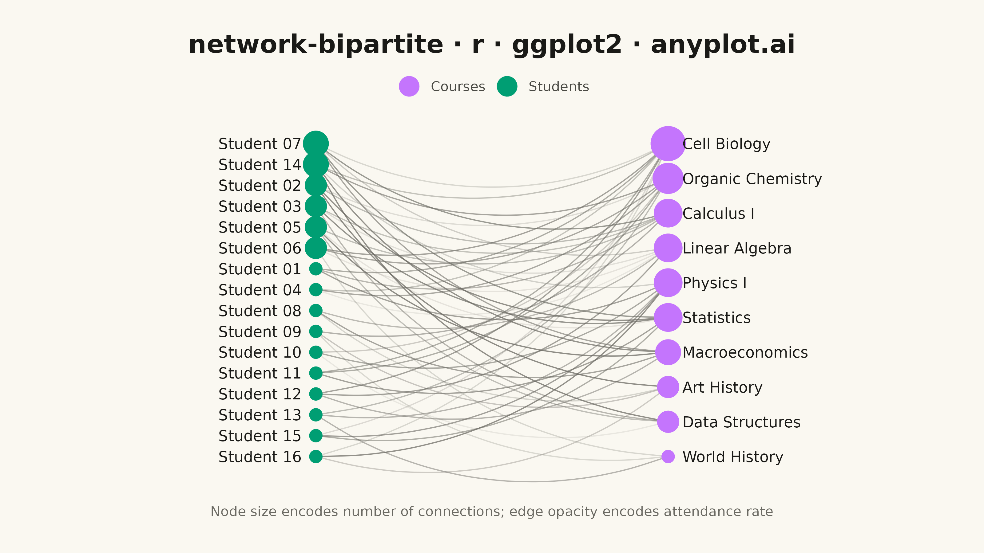
A bipartite network graph visualizes relationships between two distinct sets of entities, where edges only connect nodes from different sets — never within the same set. The two node groups are arranged in separate columns or rows, making the two-mode structure immediately apparent. This layout is fundamental for understanding cross-category relationships, revealing which entities from one set are linked to which entities in the other, and exposing patterns like hubs, clusters, and isolated nodes.
#' anyplot.ai
#' network-bipartite: Bipartite Network Graph
#' Library: ggplot2 3.5.1 | R 4.4.1
#' Quality: 92/100 | Created: 2026-09-05

library(ggplot2)
library(dplyr)
library(tidyr)
library(ragg)

set.seed(42)

# --- Theme tokens ------------------------------------------------------------
THEME       <- Sys.getenv("ANYPLOT_THEME", "light")
PAGE_BG     <- if (THEME == "light") "#FAF8F1" else "#1A1A17"
INK         <- if (THEME == "light") "#1A1A17" else "#F0EFE8"
INK_SOFT    <- if (THEME == "light") "#4A4A44" else "#B8B7B0"
INK_MUTED   <- if (THEME == "light") "#6B6A63" else "#A8A79F"
IMPRINT_PALETTE <- c("#009E73", "#C475FD", "#4467A3", "#BD8233",
                      "#AE3030", "#2ABCCD", "#954477", "#99B314")

# --- Data --------------------------------------------------------------------
# Student-course enrollment: which students registered in which courses,
# with attendance rate as the edge weight.
students <- sprintf("Student %02d", 1:16)
courses <- c("Calculus I", "Linear Algebra", "Data Structures", "Organic Chemistry",
             "Cell Biology", "Macroeconomics", "Art History", "Statistics",
             "Physics I", "World History")

edges <- bind_rows(lapply(students, function(s) {
  chosen <- sample(courses, sample(3:5, 1))
  tibble(source = s, target = chosen, weight = round(runif(length(chosen), 0.5, 1.0), 2))
}))

student_degree <- tibble(node = students) %>%
  left_join(count(edges, source, name = "degree"), by = c("node" = "source")) %>%
  mutate(degree = replace_na(degree, 0))

course_degree <- tibble(node = courses) %>%
  left_join(count(edges, target, name = "degree"), by = c("node" = "target")) %>%
  mutate(degree = replace_na(degree, 0))

# Two fixed columns, nodes ordered by degree so hubs cluster near the top.
students_pos <- student_degree %>%
  arrange(desc(degree), node) %>%
  mutate(x = 0, y = seq(1, 0, length.out = n()), set = "Students")

courses_pos <- course_degree %>%
  arrange(desc(degree), node) %>%
  mutate(x = 1, y = seq(1, 0, length.out = n()), set = "Courses")

nodes <- bind_rows(students_pos, courses_pos)

edge_coords <- edges %>%
  left_join(students_pos %>% select(node, x, y), by = c("source" = "node")) %>%
  rename(x_start = x, y_start = y) %>%
  left_join(courses_pos %>% select(node, x, y), by = c("target" = "node")) %>%
  rename(x_end = x, y_end = y)

# --- Plot ----------------------------------------------------------------
p <- ggplot() +
  geom_curve(
    data = edge_coords,
    aes(x = x_start, y = y_start, xend = x_end, yend = y_end, alpha = weight),
    color = INK_MUTED, linewidth = 0.35, curvature = 0.25, ncp = 8
  ) +
  geom_point(data = nodes, aes(x = x, y = y, size = degree, color = set)) +
  geom_text(
    data = students_pos, aes(x = x, y = y, label = node),
    hjust = 1, nudge_x = -0.04, size = 3.1, color = INK
  ) +
  geom_text(
    data = courses_pos, aes(x = x, y = y, label = node),
    hjust = 0, nudge_x = 0.04, size = 3.1, color = INK
  ) +
  scale_color_manual(values = c("Students" = IMPRINT_PALETTE[1], "Courses" = IMPRINT_PALETTE[2]),
                      name = NULL) +
  scale_size_continuous(range = c(3, 9), guide = "none") +
  scale_alpha_continuous(range = c(0.12, 0.75), guide = "none") +
  coord_cartesian(xlim = c(-0.55, 1.55), ylim = c(-0.05, 1.05), clip = "off") +
  labs(
    title = "network-bipartite · r · ggplot2 · anyplot.ai",
    caption = "Node size encodes number of connections; edge opacity encodes attendance rate"
  ) +
  guides(color = guide_legend(override.aes = list(size = 5))) +
  theme_void(base_size = 8) +
  theme(
    plot.background  = element_rect(fill = PAGE_BG, color = PAGE_BG),
    panel.background = element_rect(fill = PAGE_BG, color = NA),
    plot.title       = element_text(color = INK, size = 15, face = "bold", hjust = 0.5, margin = margin(b = 8)),
    plot.caption     = element_text(color = INK_MUTED, size = 8, hjust = 0.5, margin = margin(t = 10)),
    legend.position  = "top",
    legend.text      = element_text(color = INK_SOFT, size = 8),
    legend.key       = element_rect(fill = PAGE_BG, color = NA),
    plot.margin      = margin(t = 20, r = 50, b = 20, l = 50)
  )

# --- Save --------------------------------------------------------------------
ggsave(
  filename = sprintf("plot-%s.png", THEME),
  plot     = p,
  device   = ragg::agg_png,
  width    = 8,
  height   = 4.5,
  units    = "in",
  dpi      = 400
)
Runnable source as JSON, for any HTTP client: https://api.anyplot.ai/specs/network-bipartite/ggplot2/code. Any spec id and library id listed in llms-full.txt fit the same URL shape; every URL below is complete and callable.
{
  "spec_id": "network-bipartite",
  "language": "r",
  "library": "ggplot2",
  "page": "https://anyplot.ai/network-bipartite/r/ggplot2",
  "hub": "https://anyplot.ai/network-bipartite",
  "code_json": "https://api.anyplot.ai/specs/network-bipartite/ggplot2/code",
  "spec_json": "https://api.anyplot.ai/specs/network-bipartite",
  "render_light_png": "https://storage.googleapis.com/anyplot-images/plots/network-bipartite/r/ggplot2/plot-light.png",
  "render_dark_png": "https://storage.googleapis.com/anyplot-images/plots/network-bipartite/r/ggplot2/plot-dark.png",
  "quality_score": 92.0,
  "license": "MIT",
  "guide": "https://anyplot.ai/llms.txt"
}
Part of Bipartite Network Graph on anyplot.ai.