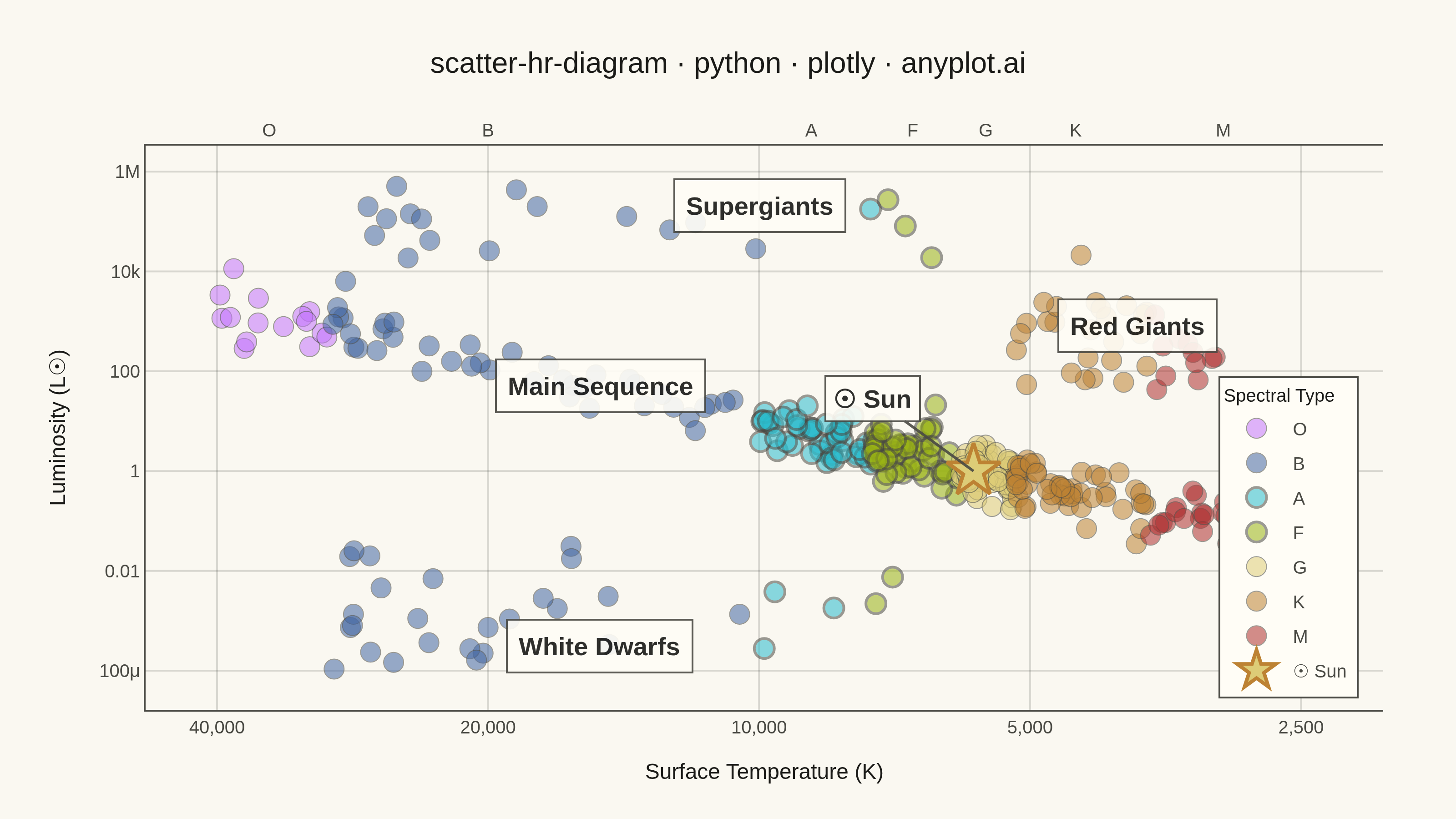
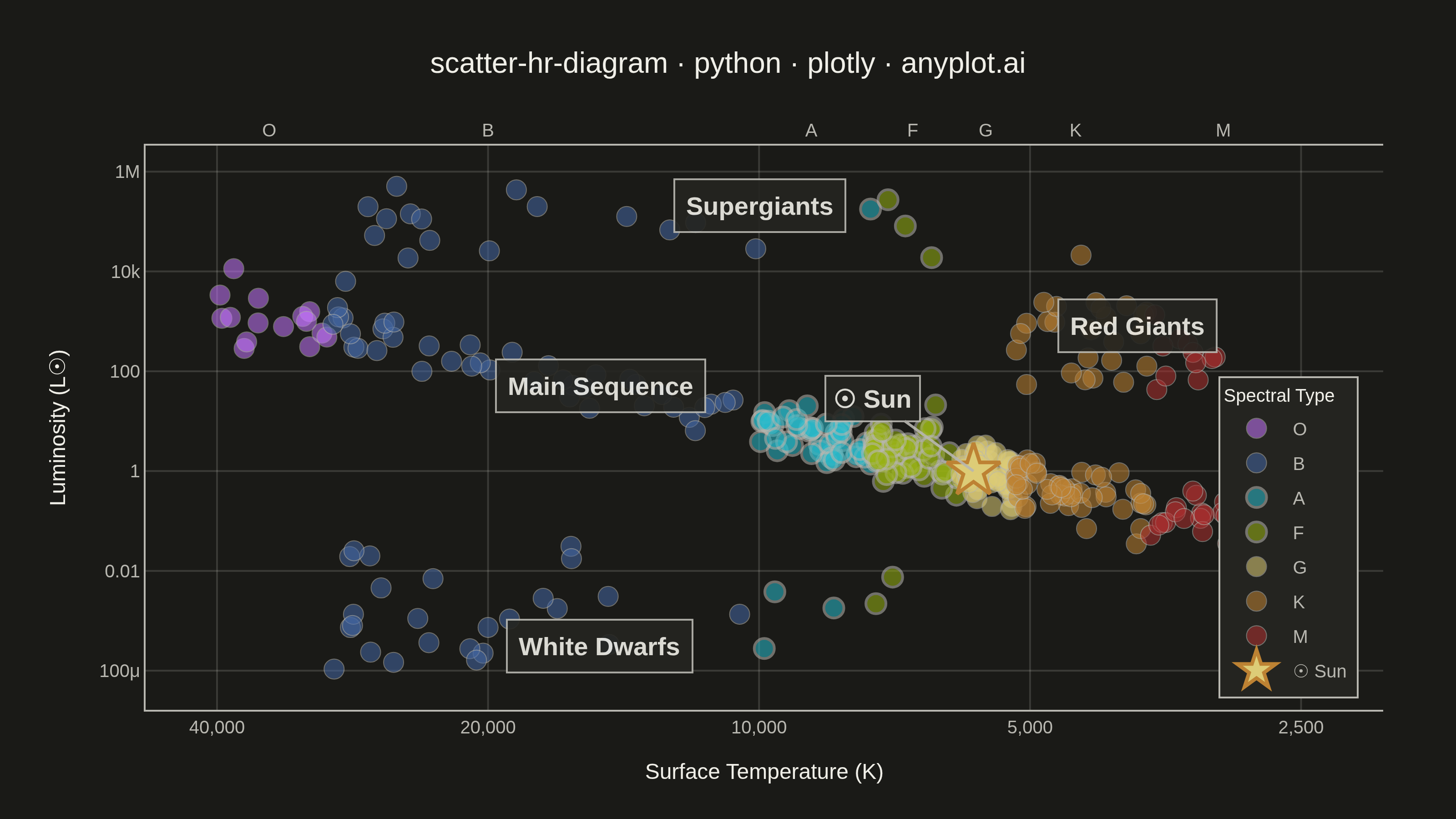
The Hertzsprung-Russell (HR) diagram is the iconic astrophysics scatter plot that shows stellar luminosity (or absolute magnitude) versus surface temperature (or spectral class). Stars naturally cluster along the main sequence diagonal, with distinct regions for red giants, supergiants, and white dwarfs, revealing the fundamental relationship between stellar temperature and brightness.
""" anyplot.ai
scatter-hr-diagram: Hertzsprung-Russell Diagram
Library: plotly 6.7.0 | Python 3.13.13
Quality: 91/100 | Updated: 2026-06-02
"""

import os

import numpy as np
import plotly.graph_objects as go


# Theme tokens (Imprint palette + theme-adaptive chrome)
THEME = os.getenv("ANYPLOT_THEME", "light")
PAGE_BG = "#FAF8F1" if THEME == "light" else "#1A1A17"
ELEVATED_BG = "#FFFDF6" if THEME == "light" else "#242420"
INK = "#1A1A17" if THEME == "light" else "#F0EFE8"
INK_SOFT = "#4A4A44" if THEME == "light" else "#B8B7B0"
GRID = "rgba(26,26,23,0.15)" if THEME == "light" else "rgba(240,239,232,0.15)"

# Domain-appropriate spectral colors using closest Imprint palette members (semantic exception to canonical order)
ANYPLOT_AMBER = "#DDCC77"  # warm-yellow anchor — used for G-type (sun-like golden)
spectral_config = {
    "O": {"temp": (30000, 40000), "color": "#C475FD", "n": 15},  # Imprint lavender (violet, hottest)
    "B": {"temp": (10000, 30000), "color": "#4467A3", "n": 40},  # Imprint blue
    "A": {"temp": (7500, 10000), "color": "#2ABCCD", "n": 45},  # Imprint cyan (blue-white)
    "F": {"temp": (6000, 7500), "color": "#99B314", "n": 50},  # Imprint lime (white-yellow)
    "G": {"temp": (5200, 6000), "color": ANYPLOT_AMBER, "n": 55},  # amber anchor (golden, sun-like)
    "K": {"temp": (3700, 5200), "color": "#BD8233", "n": 50},  # Imprint ochre (orange)
    "M": {"temp": (2400, 3700), "color": "#AE3030", "n": 45},  # Imprint matte red (coolest)
}

# Data
np.random.seed(42)

temperatures = []
luminosities = []
spectral_types = []

# Main sequence stars (L ~ T^4 relationship with scatter)
for stype, cfg in spectral_config.items():
    n = cfg["n"]
    temp = np.random.uniform(cfg["temp"][0], cfg["temp"][1], n)
    log_lum_base = 4.0 * np.log10(temp / 5778)
    log_lum = log_lum_base + np.random.normal(0, 0.3, n)
    temperatures.extend(temp)
    luminosities.extend(10**log_lum)
    spectral_types.extend([stype] * n)

# Red giants (cool but bright)
n_rg = 35
rg_temp = np.random.uniform(3000, 5200, n_rg)
rg_lum = 10 ** np.random.uniform(1.5, 3.5, n_rg)
temperatures.extend(rg_temp)
luminosities.extend(rg_lum)
spectral_types.extend(np.where(rg_temp > 3700, "K", "M").tolist())

# Supergiants (bright across temperatures) — classify without helper function
n_sg = 20
sg_temp = np.random.uniform(3500, 30000, n_sg)
sg_lum = 10 ** np.random.uniform(4.0, 5.8, n_sg)
temperatures.extend(sg_temp)
luminosities.extend(sg_lum)
spectral_types.extend(
    np.select(
        [sg_temp > 30000, sg_temp > 10000, sg_temp > 7500, sg_temp > 6000, sg_temp > 5200, sg_temp > 3700],
        ["O", "B", "A", "F", "G", "K"],
        default="M",
    ).tolist()
)

# White dwarfs (hot but dim) — classify without helper function
n_wd = 30
wd_temp = np.random.uniform(7000, 30000, n_wd)
wd_lum = 10 ** np.random.uniform(-4, -1.5, n_wd)
temperatures.extend(wd_temp)
luminosities.extend(wd_lum)
spectral_types.extend(
    np.select(
        [wd_temp > 30000, wd_temp > 10000, wd_temp > 7500, wd_temp > 6000, wd_temp > 5200, wd_temp > 3700],
        ["O", "B", "A", "F", "G", "K"],
        default="M",
    ).tolist()
)

temperatures = np.array(temperatures)
luminosities = np.array(luminosities)
spectral_types = np.array(spectral_types)

spectral_colors = {k: v["color"] for k, v in spectral_config.items()}

# Plot
fig = go.Figure()

spectral_order = ["O", "B", "A", "F", "G", "K", "M"]
for stype in spectral_order:
    mask = spectral_types == stype
    # A (#2ABCCD) and F (#99B314) get thicker stroke for extra contrast on light background
    stroke_width = 1.5 if stype in ("A", "F") else 0.5
    fig.add_trace(
        go.Scatter(
            x=temperatures[mask],
            y=luminosities[mask],
            mode="markers",
            name=stype,
            marker={
                "size": 11,
                "color": spectral_colors[stype],
                "line": {"width": stroke_width, "color": INK_SOFT},
                "opacity": 0.55,
            },
            hovertemplate=(
                f"Spectral Type: {stype}<br>Temperature: %{{x:,.0f}} K<br>Luminosity: %{{y:.4g}} L☉<br><extra></extra>"
            ),
        )
    )

# Sun reference point — star focal point using G-type color
fig.add_trace(
    go.Scatter(
        x=[5778],
        y=[1.0],
        mode="markers",
        name="☉ Sun",
        marker={"size": 22, "color": ANYPLOT_AMBER, "line": {"width": 2, "color": "#BD8233"}, "symbol": "star"},
        hovertemplate="The Sun<br>Temperature: 5,778 K<br>Luminosity: 1.0 L☉<br><extra></extra>",
    )
)

# Sun label annotation with arrow (log10 coords required for log-type axes in Plotly)
fig.add_annotation(
    x=np.log10(5778),
    y=np.log10(1.0),
    xref="x",
    yref="y",
    text="<b>☉ Sun</b>",
    showarrow=True,
    arrowhead=0,
    arrowwidth=1.5,
    arrowcolor=INK_SOFT,
    ax=-55,
    ay=-40,
    font={"size": 14, "color": INK},
    bgcolor=ELEVATED_BG,
    bordercolor=INK_SOFT,
    borderpad=4,
    opacity=0.9,
)

# Region label annotations (theme-adaptive backgrounds)
region_labels = {
    "Main Sequence": {"x": 15000, "y": 50},
    "Red Giants": {"x": 3800, "y": 800},
    "Supergiants": {"x": 10000, "y": 200000},
    "White Dwarfs": {"x": 15000, "y": 0.0003},
}

for label, pos in region_labels.items():
    fig.add_annotation(
        x=np.log10(pos["x"]),
        y=np.log10(pos["y"]),
        xref="x",
        yref="y",
        text=f"<b>{label}</b>",
        showarrow=False,
        font={"size": 14, "color": INK},
        bgcolor=ELEVATED_BG,
        bordercolor=INK_SOFT,
        borderwidth=1,
        borderpad=6,
        opacity=0.9,
    )

# Secondary x-axis with spectral class labels
spectral_temps = {"O": 35000, "B": 20000, "A": 8750, "F": 6750, "G": 5600, "K": 4450, "M": 3050}

# Empty trace to activate xaxis2
fig.add_trace(go.Scatter(x=[], y=[], xaxis="x2", showlegend=False, hoverinfo="skip"))

title = "scatter-hr-diagram · python · plotly · anyplot.ai"

# Layout — canvas 800×450 at scale=4 → 3200×1800 px output
fig.update_layout(
    autosize=False,
    paper_bgcolor=PAGE_BG,
    plot_bgcolor=PAGE_BG,
    title={"text": title, "font": {"size": 16, "color": INK}, "x": 0.5, "xanchor": "center"},
    xaxis={
        "title": {"text": "Surface Temperature (K)", "font": {"size": 12, "color": INK}},
        "tickfont": {"size": 10, "color": INK_SOFT},
        "type": "log",
        "autorange": "reversed",
        "showgrid": True,
        "gridcolor": GRID,
        "gridwidth": 1,
        "showline": True,
        "linecolor": INK_SOFT,
        "linewidth": 1,
        "mirror": False,
        "tickvals": [2500, 5000, 10000, 20000, 40000],
        "ticktext": ["2,500", "5,000", "10,000", "20,000", "40,000"],
    },
    yaxis={
        "title": {"text": "Luminosity (L☉)", "font": {"size": 12, "color": INK}},
        "tickfont": {"size": 10, "color": INK_SOFT},
        "type": "log",
        "showgrid": True,
        "gridcolor": GRID,
        "gridwidth": 1,
        "showline": True,
        "linecolor": INK_SOFT,
        "linewidth": 1,
        "mirror": False,
    },
    xaxis2={
        "tickfont": {"size": 10, "color": INK_SOFT},
        "overlaying": "x",
        "side": "top",
        "type": "log",
        "range": [np.log10(45000), np.log10(2000)],
        "tickvals": list(spectral_temps.values()),
        "ticktext": list(spectral_temps.keys()),
        "showgrid": False,
        "showline": True,
        "linecolor": INK_SOFT,
        "linewidth": 1,
        "matches": "x",
    },
    legend={
        "title": {"text": "Spectral Type", "font": {"size": 10, "color": INK}},
        "font": {"size": 10, "color": INK_SOFT},
        "bgcolor": ELEVATED_BG,
        "bordercolor": INK_SOFT,
        "borderwidth": 1,
        "x": 0.98,
        "y": 0.02,
        "xanchor": "right",
        "yanchor": "bottom",
    },
    margin={"l": 80, "r": 40, "t": 80, "b": 60},
)

# Save — 3200×1800 landscape (width=800, height=450, scale=4)
fig.write_image(f"plot-{THEME}.png", width=800, height=450, scale=4)
fig.write_html(f"plot-{THEME}.html", include_plotlyjs="cdn")
Runnable source as JSON, for any HTTP client: https://api.anyplot.ai/specs/scatter-hr-diagram/plotly/code. Any spec id and library id listed in llms-full.txt fit the same URL shape; every URL below is complete and callable.
{
  "spec_id": "scatter-hr-diagram",
  "language": "python",
  "library": "plotly",
  "page": "https://anyplot.ai/scatter-hr-diagram/python/plotly",
  "hub": "https://anyplot.ai/scatter-hr-diagram",
  "code_json": "https://api.anyplot.ai/specs/scatter-hr-diagram/plotly/code",
  "spec_json": "https://api.anyplot.ai/specs/scatter-hr-diagram",
  "render_light_png": "https://storage.googleapis.com/anyplot-images/plots/scatter-hr-diagram/python/plotly/plot-light.png",
  "render_dark_png": "https://storage.googleapis.com/anyplot-images/plots/scatter-hr-diagram/python/plotly/plot-dark.png",
  "interactive_light_html": "https://storage.googleapis.com/anyplot-images/plots/scatter-hr-diagram/python/plotly/plot-light.html",
  "interactive_dark_html": "https://storage.googleapis.com/anyplot-images/plots/scatter-hr-diagram/python/plotly/plot-dark.html",
  "quality_score": 91.0,
  "license": "MIT",
  "guide": "https://anyplot.ai/llms.txt"
}
Part of Hertzsprung-Russell Diagram on anyplot.ai.