The same plot in 14 other libraries — Python: Altair, Bokeh, lets-plot, Matplotlib, Plotly, plotnine, Pygal, Seaborn; Julia: Makie.jl; JavaScript: Chart.js, D3.js, Apache ECharts, Highcharts, MUI X Charts. Compare all 15 side by side: Hertzsprung-Russell Diagram in Python, R, Julia and JavaScript.
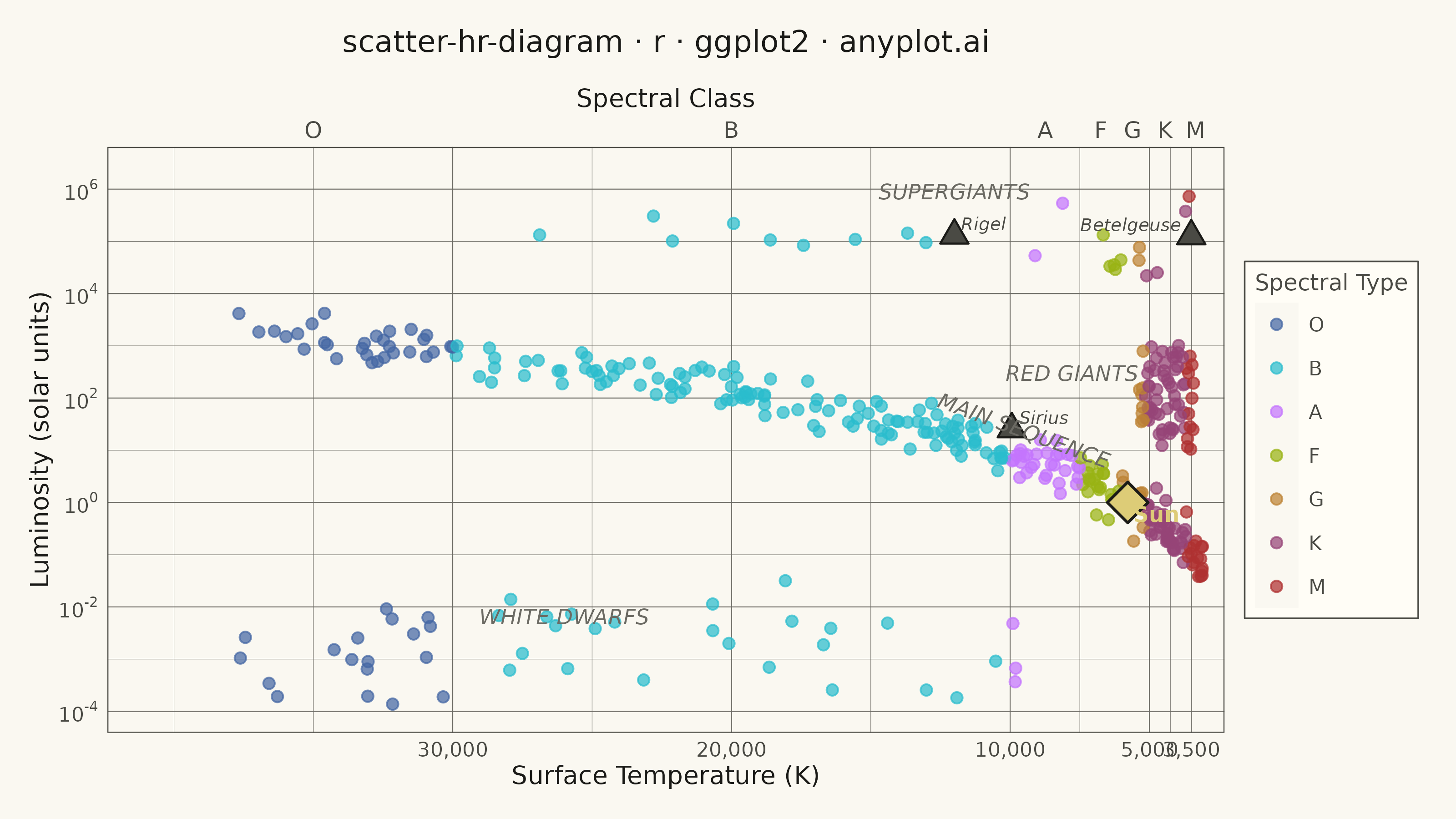
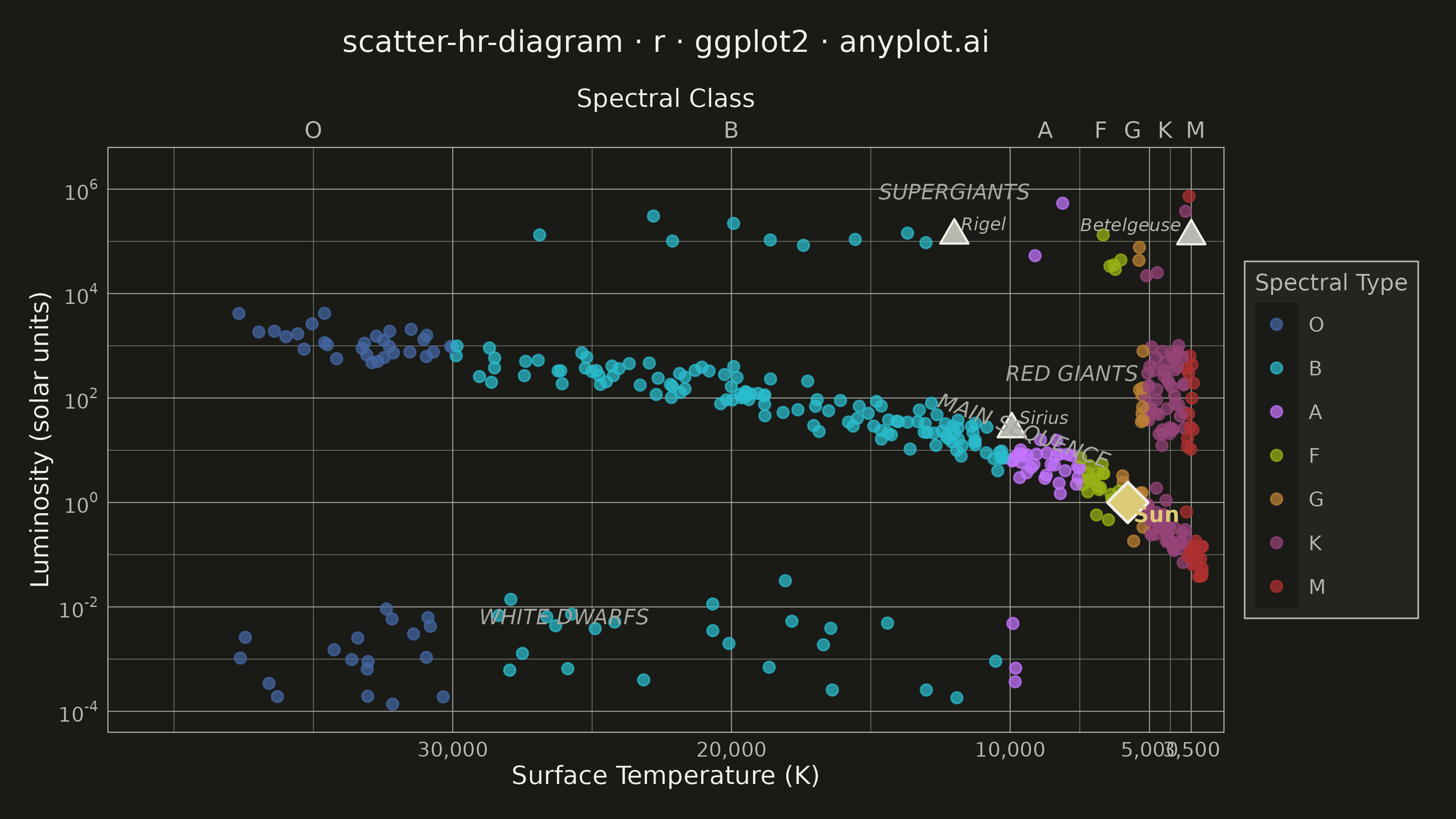
The Hertzsprung-Russell (HR) diagram is the iconic astrophysics scatter plot that shows stellar luminosity (or absolute magnitude) versus surface temperature (or spectral class). Stars naturally cluster along the main sequence diagonal, with distinct regions for red giants, supergiants, and white dwarfs, revealing the fundamental relationship between stellar temperature and brightness.
#' anyplot.ai
#' scatter-hr-diagram: Hertzsprung-Russell Diagram
#' Library: ggplot2 3.5.1 | R 4.4.1
#' Quality: 86/100 | Created: 2026-06-02

library(ggplot2)
library(scales)
library(ragg)

set.seed(42)

# --- Theme tokens -----------------------------------------------------------
THEME       <- Sys.getenv("ANYPLOT_THEME", "light")
PAGE_BG     <- if (THEME == "light") "#FAF8F1" else "#1A1A17"
ELEVATED_BG <- if (THEME == "light") "#FFFDF6" else "#242420"
INK         <- if (THEME == "light") "#1A1A17" else "#F0EFE8"
INK_SOFT    <- if (THEME == "light") "#4A4A44" else "#B8B7B0"
INK_MUTED   <- if (THEME == "light") "#6B6A63" else "#A8A79F"

# Spectral type colors — semantic exception: conventional stellar color sequence
# O/B are blue, A is pale lavender (white-ish), F/G are warm yellow-ochre,
# K is rose (nearest Imprint to orange), M is matte red — all Imprint palette
SPECTRAL_COLORS <- c(
    "O" = "#4467A3",  # blue — O stars are intensely blue-hot
    "B" = "#2ABCCD",  # cyan — B stars are blue-white
    "A" = "#C475FD",  # lavender — A stars are white/pale blue-white
    "F" = "#99B314",  # lime — F stars are yellow-white
    "G" = "#BD8233",  # ochre — G stars are yellow (Sun-like)
    "K" = "#954477",  # rose — K stars are orange-red
    "M" = "#AE3030"   # matte red — M stars are red
)

# Assign spectral type based on effective temperature (Harvard classification)
spectral_class <- function(temp) {
    ifelse(temp >= 30000, "O",
    ifelse(temp >= 10000, "B",
    ifelse(temp >= 7500,  "A",
    ifelse(temp >= 6000,  "F",
    ifelse(temp >= 5200,  "G",
    ifelse(temp >= 3700,  "K", "M"))))))
}

# --- Data -------------------------------------------------------------------
# Main sequence: luminosity ~ T^4 (Stefan-Boltzmann), log-linear with scatter
n_ms    <- 280
ms_temp <- 10^runif(n_ms, log10(3100), log10(38000))
ms_lum  <- 10^(4.0 * (log10(ms_temp) - log10(5778)) + rnorm(n_ms, sd = 0.25))

# Red giants: evolved stars — cool, moderately luminous
n_rg    <- 70
rg_temp <- runif(n_rg, 3400, 5400)
rg_lum  <- 10^(runif(n_rg, 1.2, 2.9) + rnorm(n_rg, sd = 0.12))

# Supergiants: extremely luminous across wide temperature range
n_sg    <- 22
sg_temp <- c(runif(11, 3500, 7000), runif(11, 8000, 28000))
sg_lum  <- 10^(runif(n_sg, 4.3, 5.8) + rnorm(n_sg, sd = 0.18))

# White dwarfs: hot but very dim — compact degenerate remnants
n_wd    <- 45
wd_temp <- runif(n_wd, 9000, 38000)
wd_lum  <- 10^(runif(n_wd, -3.8, -1.6) + rnorm(n_wd, sd = 0.18))

# Combined stellar dataset with spectral type and region classification
all_temp <- c(ms_temp, rg_temp, sg_temp, wd_temp)
all_lum  <- c(ms_lum,  rg_lum,  sg_lum,  wd_lum)
all_reg  <- c(rep("Main Sequence", n_ms), rep("Red Giants", n_rg),
              rep("Supergiants",   n_sg), rep("White Dwarfs", n_wd))

df <- data.frame(
    temperature   = all_temp,
    luminosity    = all_lum,
    region        = factor(all_reg, levels = c("Main Sequence", "Red Giants",
                                               "Supergiants", "White Dwarfs")),
    spectral_type = factor(spectral_class(all_temp),
                           levels = c("O", "B", "A", "F", "G", "K", "M"))
)

# Sun: reference star — 5,778 K, 1.0 L_sun, G2V spectral type
sun <- data.frame(temperature = 5778, luminosity = 1.0)

# Notable named stars (star_name data dimension — DQ-01)
named_stars <- data.frame(
    temperature = c(3500,   9940,  12000),
    luminosity  = c(1.26e5, 25.4,  1.3e5),
    star_name   = c("Betelgeuse", "Sirius", "Rigel")
)

# --- Plot -------------------------------------------------------------------
title_str <- "scatter-hr-diagram · r · ggplot2 · anyplot.ai"

p <- ggplot(df, aes(x = temperature, y = luminosity, color = spectral_type)) +
    geom_point(size = 1.8, alpha = 0.72) +
    # Sun: amber filled diamond — distinct reference marker
    geom_point(
        data        = sun,
        aes(x = temperature, y = luminosity),
        color       = INK,
        fill        = "#DDCC77",
        size        = 5.5,
        shape       = 23,
        stroke      = 0.8,
        inherit.aes = FALSE
    ) +
    # Named star markers (filled triangles to distinguish from scatter)
    geom_point(
        data        = named_stars,
        aes(x = temperature, y = luminosity),
        color       = INK,
        fill        = INK_SOFT,
        size        = 3.5,
        shape       = 24,
        stroke      = 0.6,
        inherit.aes = FALSE
    ) +
    # Named star labels
    geom_text(
        data        = named_stars,
        aes(x = temperature, y = luminosity, label = star_name),
        color       = INK_SOFT,
        size        = 2.5,
        fontface    = "italic",
        hjust       = c(1.1, -0.15, -0.15),
        vjust       = -0.4,
        inherit.aes = FALSE
    ) +
    # Stellar region annotations guide the viewer through populations
    annotate("text",
        x = 12000, y = 9e5,
        label = "SUPERGIANTS", color = INK_MUTED,
        size = 3.0, fontface = "italic"
    ) +
    annotate("text",
        x = 5400, y = 300,
        label = "RED GIANTS", color = INK_MUTED,
        size = 3.0, fontface = "italic", hjust = 1
    ) +
    annotate("text",
        x = 9500, y = 24,
        label = "MAIN SEQUENCE", color = INK_MUTED,
        size = 3.0, fontface = "italic", angle = -20
    ) +
    annotate("text",
        x = 26000, y = 0.0065,
        label = "WHITE DWARFS", color = INK_MUTED,
        size = 3.0, fontface = "italic"
    ) +
    # Sun label (amber matches the diamond marker fill)
    annotate("text",
        x = 4750, y = 0.60,
        label = "Sun", color = "#DDCC77",
        size = 3.0, fontface = "bold"
    ) +
    # Reversed x-axis (astrophysical convention: hot on left, cool on right)
    # Fewer breaks at cool end to avoid label crowding
    scale_x_reverse(
        name     = "Surface Temperature (K)",
        breaks   = c(30000, 20000, 10000, 5000, 3500),
        labels   = scales::label_comma(),
        limits   = c(42000, 2700),
        expand   = c(0.01, 0),
        sec.axis = sec_axis(
            transform = ~ .,
            breaks    = c(35000, 20000, 8750, 6750, 5600, 4450, 3350),
            labels    = c("O", "B", "A", "F", "G", "K", "M"),
            name      = "Spectral Class"
        )
    ) +
    # Log-scale luminosity axis with scientific notation tick labels
    scale_y_log10(
        name   = "Luminosity (solar units)",
        breaks = 10^c(-4, -2, 0, 2, 4, 6),
        labels = scales::trans_format("log10", scales::math_format(10^.x)),
        limits = c(5e-5, 5e6),
        expand = c(0.01, 0)
    ) +
    scale_color_manual(values = SPECTRAL_COLORS, name = "Spectral Type") +
    labs(title = title_str) +
    theme_minimal(base_size = 8) +
    theme(
        plot.background   = element_rect(fill = PAGE_BG,     color = PAGE_BG),
        panel.background  = element_rect(fill = PAGE_BG,     color = NA),
        panel.grid.major  = element_line(color = INK_MUTED,  linewidth = 0.18),
        panel.grid.minor  = element_line(color = INK_MUTED,  linewidth = 0.09),
        panel.border      = element_rect(color = INK_SOFT,   fill = NA,
                                         linewidth = 0.4),
        axis.title        = element_text(color = INK,        size = 10),
        axis.text         = element_text(color = INK_SOFT,   size = 8),
        axis.title.x.top  = element_text(color = INK,        size = 10,
                                         margin = margin(b = 4)),
        axis.text.x.top   = element_text(color = INK_SOFT,   size = 9),
        plot.title        = element_text(color = INK,        size = 12,
                                         hjust = 0.5,
                                         margin = margin(b = 10)),
        legend.background = element_rect(fill = ELEVATED_BG, color = INK_SOFT,
                                         linewidth = 0.3),
        legend.text       = element_text(color = INK_SOFT,   size = 8),
        legend.title      = element_text(color = INK_SOFT,   size = 9),
        legend.key        = element_rect(fill = PAGE_BG,     color = NA),
        legend.position   = "right",
        plot.margin       = margin(12, 15, 12, 12)
    )

# --- Save -------------------------------------------------------------------
ggsave(
    filename = sprintf("plot-%s.png", THEME),
    plot     = p,
    device   = ragg::agg_png,
    width    = 8,
    height   = 4.5,
    units    = "in",
    dpi      = 400
)
Runnable source as JSON, for any HTTP client: https://api.anyplot.ai/specs/scatter-hr-diagram/ggplot2/code. Any spec id and library id listed in llms-full.txt fit the same URL shape; every URL below is complete and callable.
{
  "spec_id": "scatter-hr-diagram",
  "language": "r",
  "library": "ggplot2",
  "page": "https://anyplot.ai/scatter-hr-diagram/r/ggplot2",
  "hub": "https://anyplot.ai/scatter-hr-diagram",
  "code_json": "https://api.anyplot.ai/specs/scatter-hr-diagram/ggplot2/code",
  "spec_json": "https://api.anyplot.ai/specs/scatter-hr-diagram",
  "render_light_png": "https://storage.googleapis.com/anyplot-images/plots/scatter-hr-diagram/r/ggplot2/plot-light.png",
  "render_dark_png": "https://storage.googleapis.com/anyplot-images/plots/scatter-hr-diagram/r/ggplot2/plot-dark.png",
  "quality_score": 86.0,
  "license": "MIT",
  "guide": "https://anyplot.ai/llms.txt"
}
Part of Hertzsprung-Russell Diagram on anyplot.ai.