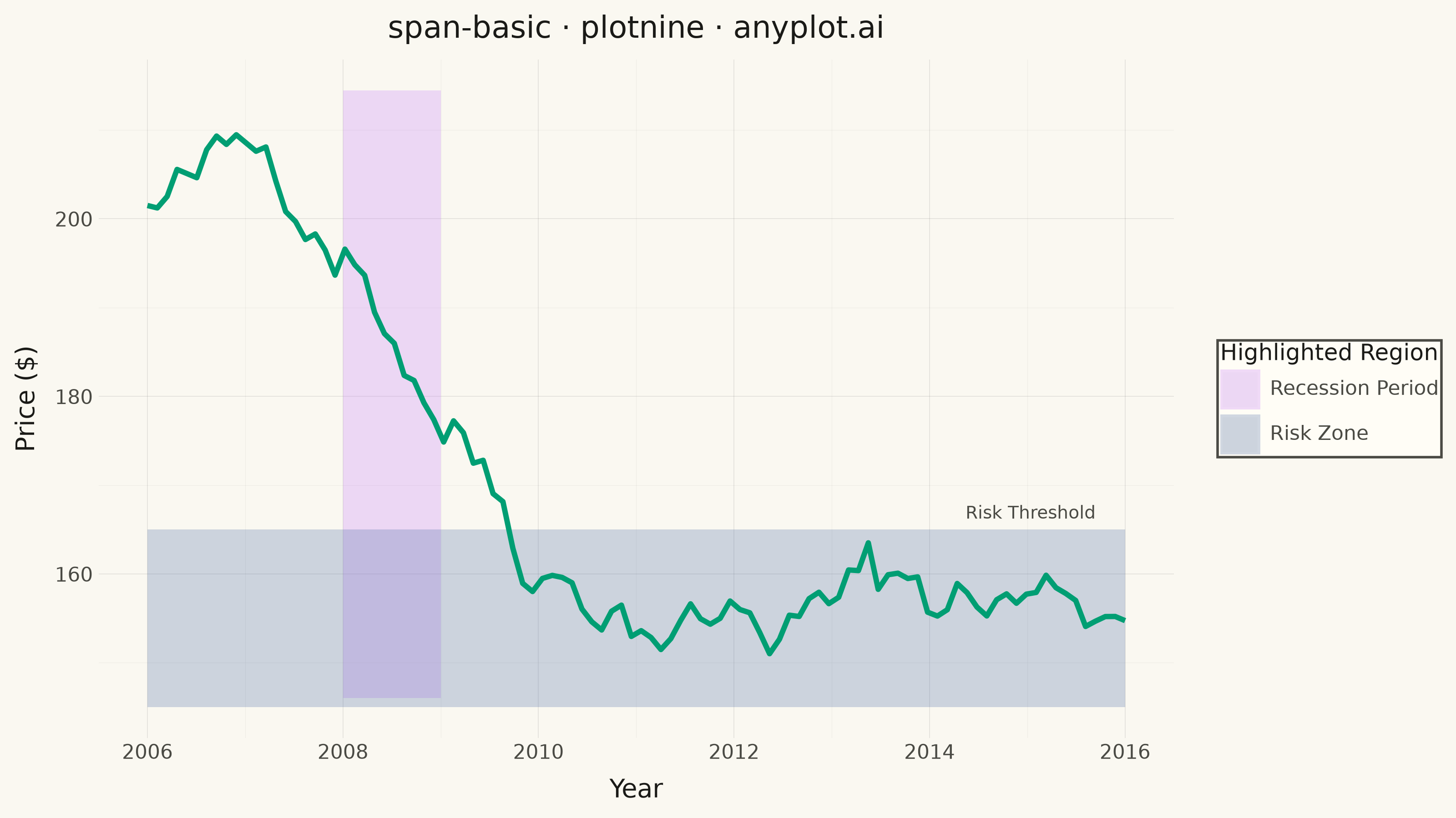
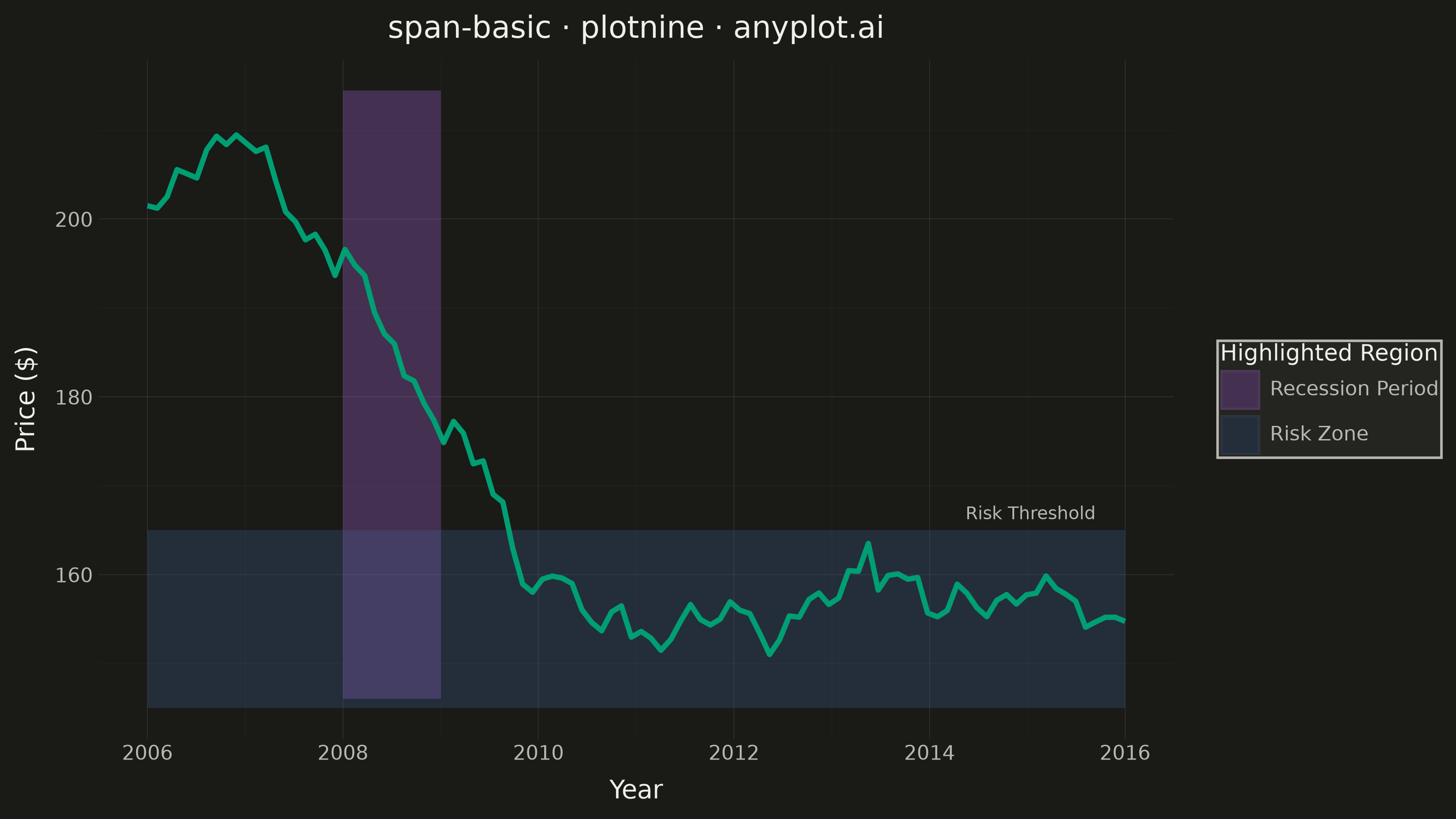
Basic Span Plot (Highlighted Region) — plotnine

A span plot highlights a specific region of interest on a chart using a shaded rectangular area that spans the full height or width of the plot. Vertical spans mark ranges along the x-axis (e.g., time periods), while horizontal spans mark ranges along the y-axis (e.g., value thresholds). The semi-transparent fill allows underlying data to remain visible while drawing attention to the highlighted region.

Basic Span Plot (Highlighted Region) rendered with plotnine

Python source (plotnine)

""" anyplot.ai
span-basic: Basic Span Plot (Highlighted Region)
Library: plotnine 0.15.7 | Python 3.13.14
Quality: 88/100 | Updated: 2026-07-25
"""

import os

import numpy as np
import pandas as pd
from plotnine import (
    aes,
    element_line,
    element_rect,
    element_text,
    geom_line,
    geom_rect,
    geom_text,
    ggplot,
    labs,
    scale_fill_manual,
    theme,
    theme_minimal,
)


# Theme tokens
THEME = os.getenv("ANYPLOT_THEME", "light")
PAGE_BG = "#FAF8F1" if THEME == "light" else "#1A1A17"
ELEVATED_BG = "#FFFDF6" if THEME == "light" else "#242420"
INK = "#1A1A17" if THEME == "light" else "#F0EFE8"
INK_SOFT = "#4A4A44" if THEME == "light" else "#B8B7B0"

IMPRINT = ["#009E73", "#C475FD", "#4467A3", "#BD8233", "#AE3030", "#2ABCCD", "#954477"]

# Data - Stock prices over 10 years with highlighted periods
np.random.seed(42)
years = np.linspace(2006, 2016, 100)
price = 100 + np.cumsum(np.random.randn(100) * 2)
recession_mask = (years >= 2008) & (years < 2010)
price[recession_mask] -= np.linspace(0, 25, recession_mask.sum())
price[years >= 2010] -= 25
price = price + np.abs(price.min()) + 50

df = pd.DataFrame({"year": years, "price": price})

y_min = df["price"].min() - 5
y_max = df["price"].max() + 5
x_min = years.min()
x_max = years.max()

spans = pd.DataFrame(
    {
        "xmin": [2008, x_min],
        "xmax": [2009, x_max],
        "ymin": [y_min, 145],
        "ymax": [y_max, 165],
        "label": ["Recession Period", "Risk Zone"],
    }
)

annotation = pd.DataFrame({"x": [x_max - 0.3], "y": [167], "text": ["Risk Threshold"]})

# Plot
plot = (
    ggplot()
    + geom_rect(data=spans, mapping=aes(xmin="xmin", xmax="xmax", ymin="ymin", ymax="ymax", fill="label"), alpha=0.25)
    + geom_line(data=df, mapping=aes(x="year", y="price"), color=IMPRINT[0], size=1.2)
    + geom_text(data=annotation, mapping=aes(x="x", y="y", label="text"), ha="right", size=7, color=INK_SOFT)
    + scale_fill_manual(values={"Recession Period": IMPRINT[1], "Risk Zone": IMPRINT[2]}, name="Highlighted Region")
    + labs(x="Year", y="Price ($)", title="span-basic · plotnine · anyplot.ai")
    + theme_minimal()
    + theme(
        figure_size=(8, 4.5),
        text=element_text(size=7),
        plot_background=element_rect(fill=PAGE_BG, color=PAGE_BG),
        panel_background=element_rect(fill=PAGE_BG),
        plot_title=element_text(size=12, color=INK),
        axis_title=element_text(size=10, color=INK),
        axis_text=element_text(size=8, color=INK_SOFT),
        legend_text=element_text(size=8, color=INK_SOFT),
        legend_title=element_text(size=9, color=INK),
        legend_background=element_rect(fill=ELEVATED_BG, color=INK_SOFT),
        panel_grid_major=element_line(color=INK, size=0.3, alpha=0.10),
        panel_grid_minor=element_line(color=INK, size=0.2, alpha=0.05),
    )
)

# Save
plot.save(f"plot-{THEME}.png", dpi=400, width=8, height=4.5, units="in", verbose=False)

Part of Basic Span Plot (Highlighted Region) on anyplot.ai.

Basic Span Plot (Highlighted Region) — plotnine

Python source (plotnine)

Other implementations