The same plot in 14 other libraries — Python: Altair, Bokeh, lets-plot, Matplotlib, Plotly, plotnine, Pygal, Seaborn; Julia: Makie.jl; JavaScript: Chart.js, D3.js, Apache ECharts, Highcharts, MUI X Charts. Compare all 15 side by side: Basic Span Plot (Highlighted Region) in Python, R, Julia and JavaScript.
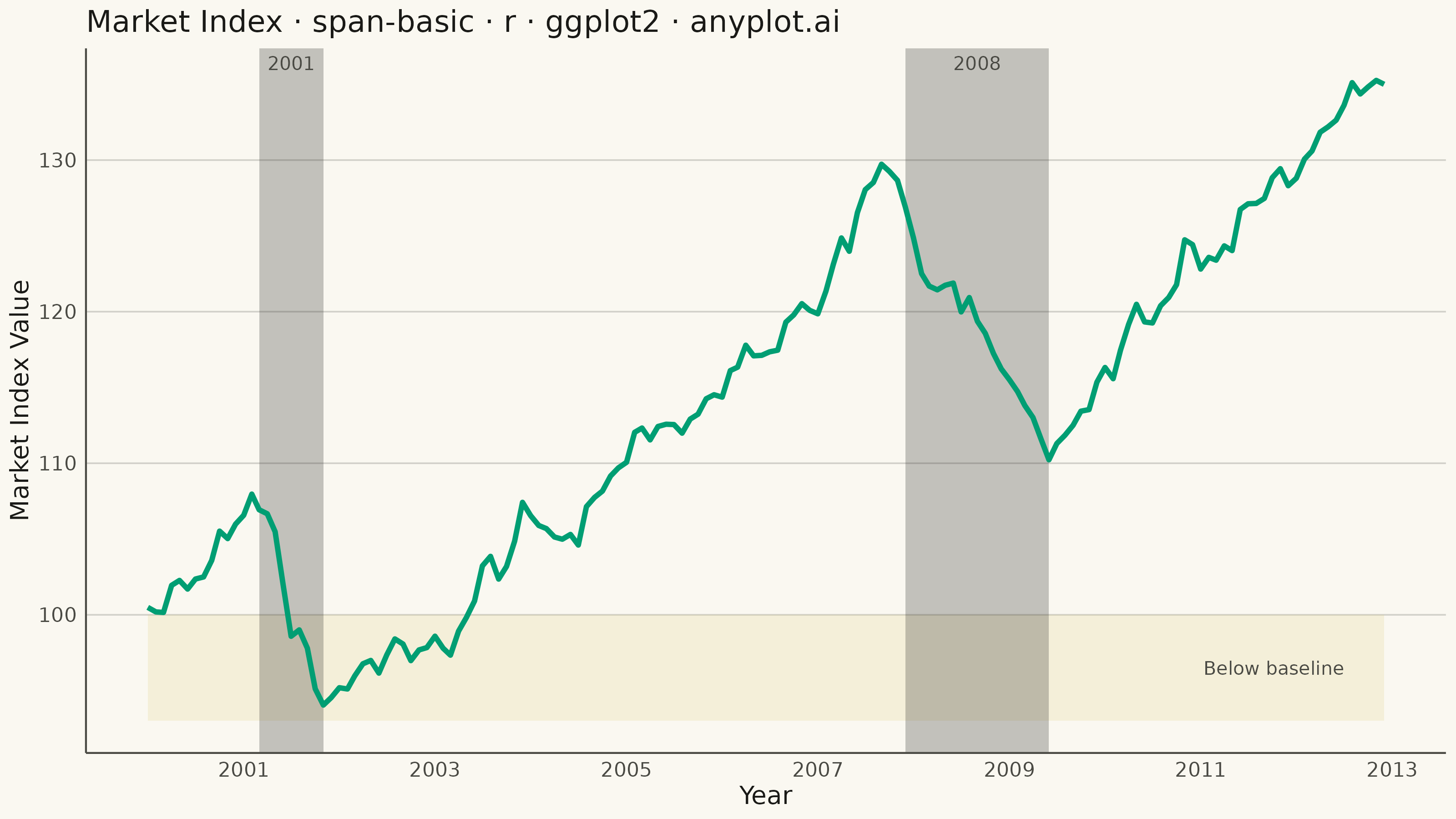
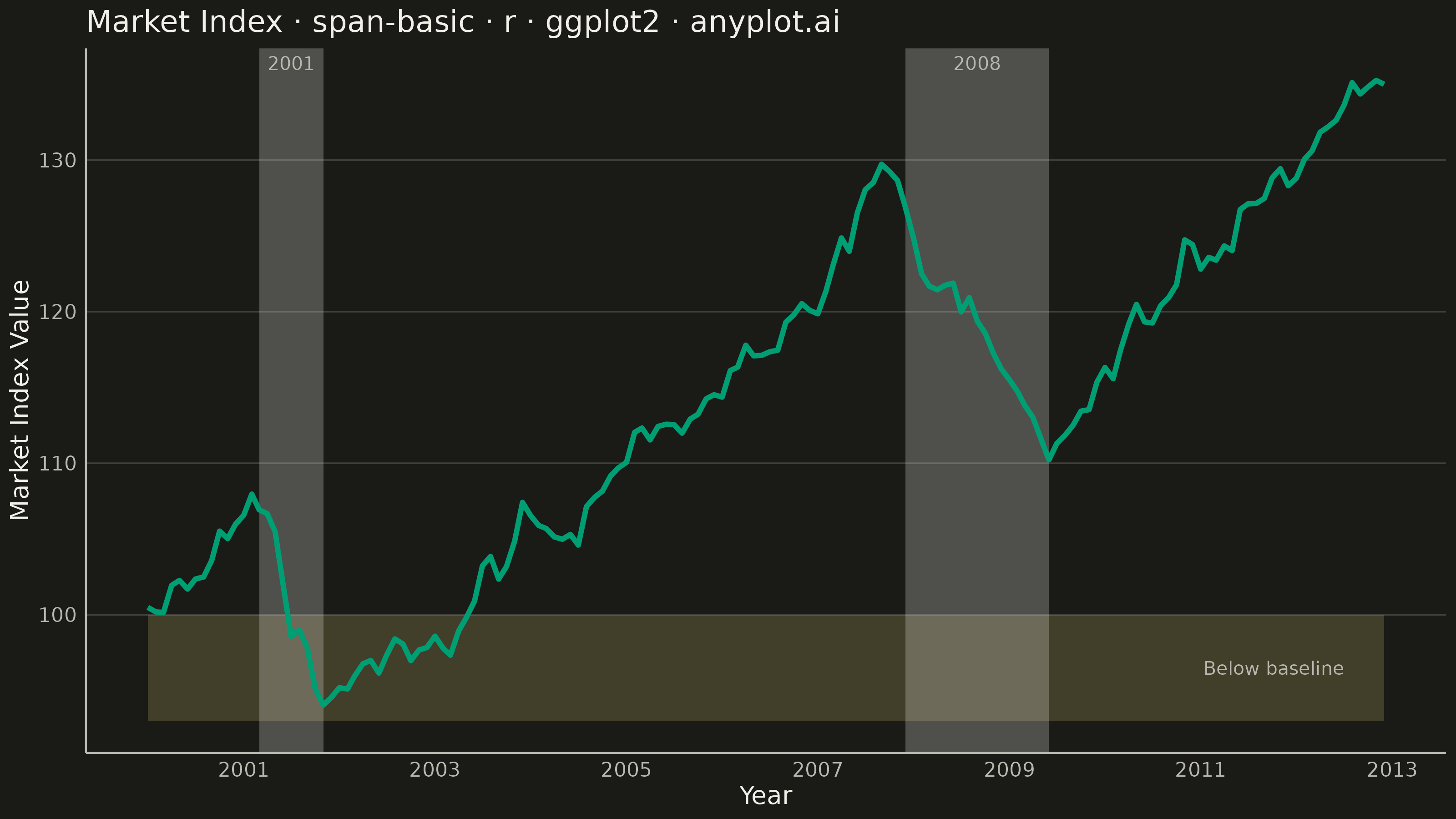
A span plot highlights a specific region of interest on a chart using a shaded rectangular area that spans the full height or width of the plot. Vertical spans mark ranges along the x-axis (e.g., time periods), while horizontal spans mark ranges along the y-axis (e.g., value thresholds). The semi-transparent fill allows underlying data to remain visible while drawing attention to the highlighted region.
#' anyplot.ai
#' span-basic: Basic Span Plot (Highlighted Region)
#' Library: ggplot2 3.5.1 | R 4.4.1
#' Quality: 92/100 | Created: 2026-07-25

library(ggplot2)
library(ragg)

set.seed(42)

# --- Theme tokens -----------------------------------------------------------
THEME       <- Sys.getenv("ANYPLOT_THEME", "light")
PAGE_BG     <- if (THEME == "light") "#FAF8F1" else "#1A1A17"
INK         <- if (THEME == "light") "#1A1A17" else "#F0EFE8"
INK_SOFT    <- if (THEME == "light") "#4A4A44" else "#B8B7B0"
NEUTRAL     <- INK  # theme-adaptive anchor for the span highlight (reference region)
AMBER       <- "#DDCC77"  # semantic anchor: warning / caution threshold band
IMPRINT_PALETTE <- c("#009E73", "#C475FD", "#4467A3", "#BD8233",
                     "#AE3030", "#2ABCCD", "#954477", "#99B314")

# ggplot2 does not expose per-element grid alpha, so blend INK toward PAGE_BG
# to get a faint tint instead of passing the full-opacity ink color.
mix_color <- function(c1, c2, amount) {
  m <- col2rgb(c1) * (1 - amount) + col2rgb(c2) * amount
  rgb(m[1, ], m[2, ], m[3, ], maxColorValue = 255)
}
GRID_COLOR <- mix_color(PAGE_BG, INK, 0.18)

# --- Data --------------------------------------------------------------------
dates <- seq(as.Date("2000-01-01"), as.Date("2012-12-01"), by = "month")
n     <- length(dates)

recessions <- tibble::tibble(
  start = as.Date(c("2001-03-01", "2007-12-01")),
  end   = as.Date(c("2001-11-01", "2009-06-01")),
  label = c("2001", "2008")
)

recession_flag <- rep(0, n)
for (i in seq_len(nrow(recessions))) {
  recession_flag <- recession_flag +
    as.numeric(dates >= recessions$start[i] & dates <= recessions$end[i])
}

monthly_step <- ifelse(recession_flag > 0,
                        rnorm(n, mean = -0.9, sd = 1.0),
                        rnorm(n, mean = 0.5, sd = 1.0))
market_index <- tibble::tibble(
  date  = dates,
  index = 100 + cumsum(monthly_step)
)

# Horizontal span: caution zone whenever the index falls below its starting
# baseline of 100 (demonstrates the spec's "horizontal" direction alongside
# the vertical recession spans above).
baseline_zone <- tibble::tibble(
  xmin = min(dates),
  xmax = max(dates),
  ymin = floor(min(market_index$index)) - 1,
  ymax = 100
)

# --- Title (scaled for length per anyplot title-fontsize rule) --------------
plot_title <- "Market Index · span-basic · r · ggplot2 · anyplot.ai"
title_size <- round(12 * min(1.0, 67 / nchar(plot_title)))
title_size <- max(title_size, 8)

# --- Plot ---------------------------------------------------------------------
p <- ggplot(market_index, aes(x = date, y = index)) +
  geom_rect(
    data        = baseline_zone,
    aes(xmin = xmin, xmax = xmax, ymin = ymin, ymax = ymax),
    inherit.aes = FALSE,
    fill        = AMBER,
    alpha       = 0.2
  ) +
  geom_rect(
    data        = recessions,
    aes(xmin = start, xmax = end, ymin = -Inf, ymax = Inf),
    inherit.aes = FALSE,
    fill        = NEUTRAL,
    alpha       = 0.25
  ) +
  geom_text(
    data        = recessions,
    aes(x = start + (end - start) / 2, y = Inf, label = label),
    inherit.aes = FALSE,
    vjust       = 1.6,
    size        = 2.6,
    color       = INK_SOFT
  ) +
  annotate(
    "text",
    x     = dates[round(n * 0.97)],
    y     = (baseline_zone$ymin + baseline_zone$ymax) / 2,
    label = "Below baseline",
    hjust = 1,
    size  = 2.6,
    color = INK_SOFT
  ) +
  geom_line(color = IMPRINT_PALETTE[1], linewidth = 1.0) +
  scale_x_date(date_breaks = "2 years", date_labels = "%Y") +
  labs(
    title = plot_title,
    x     = "Year",
    y     = "Market Index Value"
  ) +
  theme_minimal(base_size = 8) +
  theme(
    plot.background   = element_rect(fill = PAGE_BG, color = PAGE_BG),
    panel.background  = element_rect(fill = PAGE_BG, color = NA),
    panel.grid.major.x = element_blank(),
    panel.grid.major.y = element_line(color = GRID_COLOR, linewidth = 0.3),
    panel.grid.minor  = element_blank(),
    panel.border      = element_blank(),
    axis.line         = element_line(color = INK_SOFT),
    axis.ticks        = element_blank(),
    axis.title        = element_text(color = INK, size = 10),
    axis.text         = element_text(color = INK_SOFT, size = 8),
    plot.title        = element_text(color = INK, size = title_size)
  )

# --- Save ---------------------------------------------------------------------
ggsave(
  filename = sprintf("plot-%s.png", THEME),
  plot     = p,
  device   = ragg::agg_png,
  width    = 8,
  height   = 4.5,
  units    = "in",
  dpi      = 400
)
Runnable source as JSON, for any HTTP client: https://api.anyplot.ai/specs/span-basic/ggplot2/code. Any spec id and library id listed in llms-full.txt fit the same URL shape; every URL below is complete and callable.
{
  "spec_id": "span-basic",
  "language": "r",
  "library": "ggplot2",
  "page": "https://anyplot.ai/span-basic/r/ggplot2",
  "hub": "https://anyplot.ai/span-basic",
  "code_json": "https://api.anyplot.ai/specs/span-basic/ggplot2/code",
  "spec_json": "https://api.anyplot.ai/specs/span-basic",
  "render_light_png": "https://storage.googleapis.com/anyplot-images/plots/span-basic/r/ggplot2/plot-light.png",
  "render_dark_png": "https://storage.googleapis.com/anyplot-images/plots/span-basic/r/ggplot2/plot-dark.png",
  "quality_score": 92.0,
  "license": "MIT",
  "guide": "https://anyplot.ai/llms.txt"
}
Part of Basic Span Plot (Highlighted Region) on anyplot.ai.