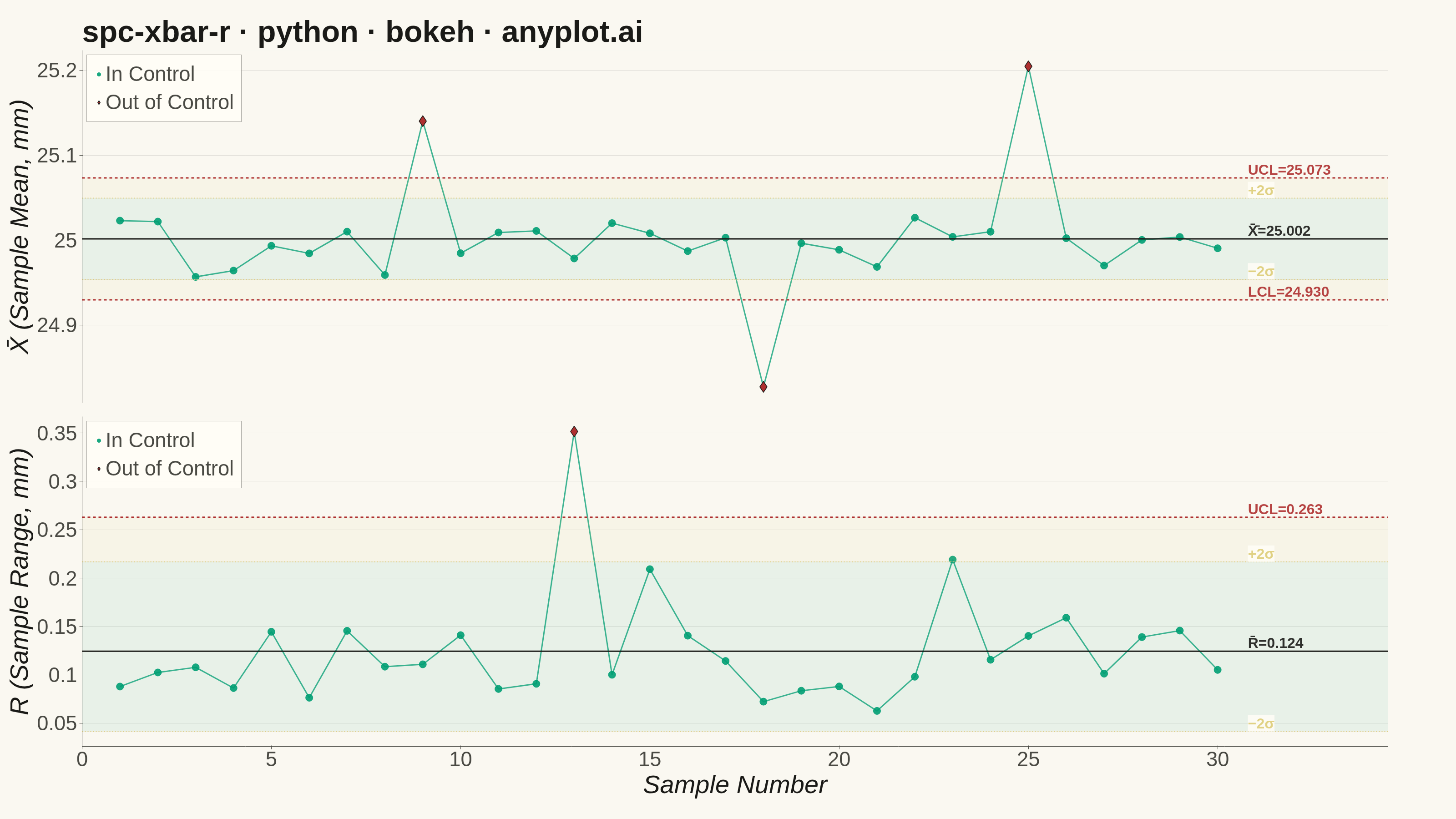
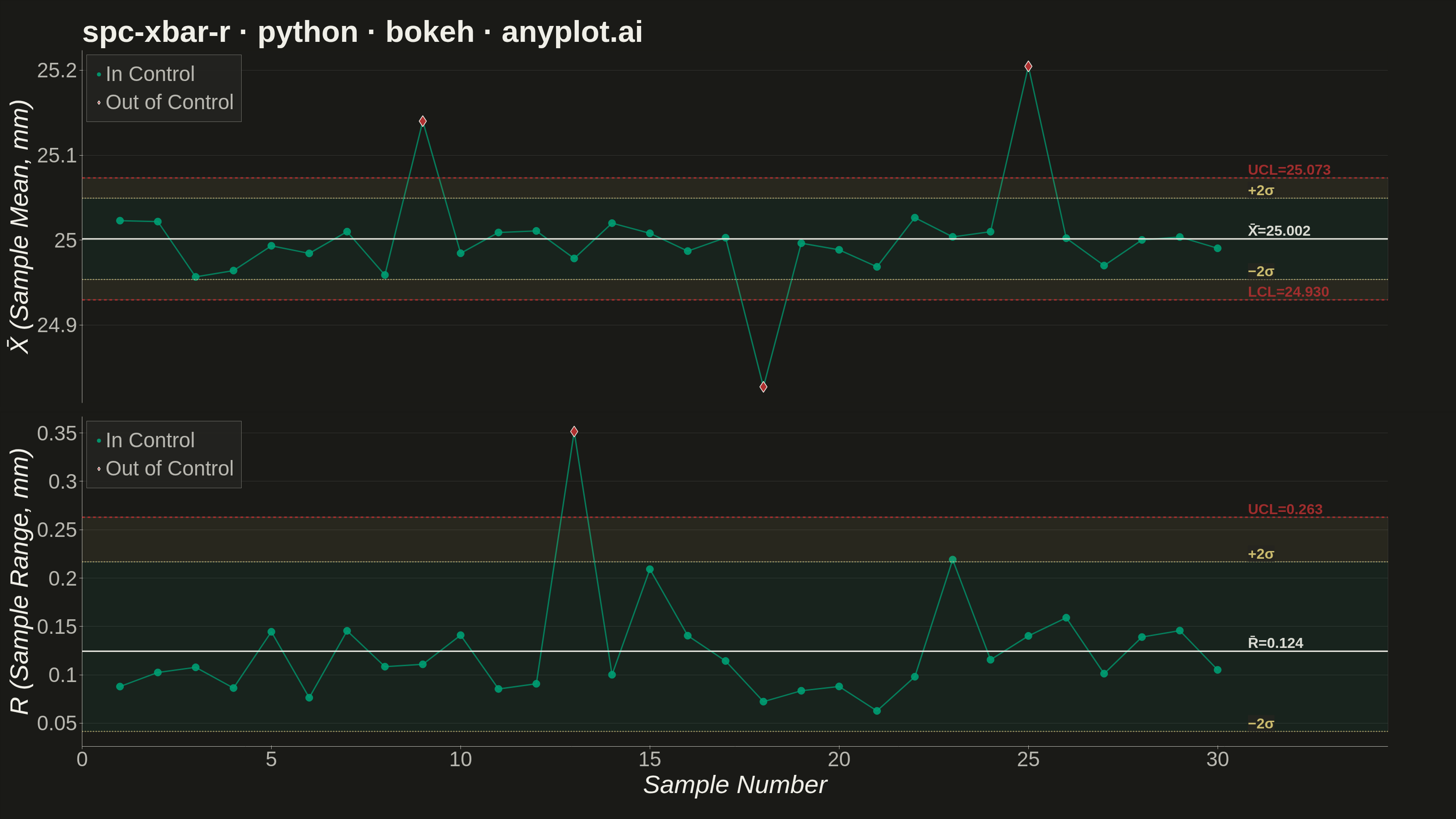
A Statistical Process Control (SPC) chart displaying sample means (X-bar) and ranges (R) plotted over time against control limits. The chart includes a center line representing the process mean, Upper Control Limit (UCL) and Lower Control Limit (LCL) at ±3 sigma, and optional warning limits at ±2 sigma. Out-of-control points are highlighted to signal process instability. This is a fundamental tool in manufacturing quality control and Six Sigma methodology for monitoring process stability.
""" anyplot.ai
spc-xbar-r: Statistical Process Control Chart (X-bar/R)
Library: bokeh 3.9.1 | Python 3.13.14
Quality: 92/100 | Updated: 2026-06-20
"""

import sys


# Remove script directory from sys.path so 'bokeh.py' doesn't shadow the installed bokeh package
if sys.path and sys.path[0] not in ("", None):
    sys.path.pop(0)

import os
import time
from pathlib import Path

import numpy as np
from bokeh.io import output_file, save
from bokeh.layouts import column
from bokeh.models import BoxAnnotation, ColumnDataSource, HoverTool, Label, Legend, LegendItem, Range1d, Span
from bokeh.plotting import figure
from selenium import webdriver
from selenium.webdriver.chrome.options import Options


# Theme-adaptive chrome tokens
THEME = os.getenv("ANYPLOT_THEME", "light")
PAGE_BG = "#FAF8F1" if THEME == "light" else "#1A1A17"
ELEVATED_BG = "#FFFDF6" if THEME == "light" else "#242420"
INK = "#1A1A17" if THEME == "light" else "#F0EFE8"
INK_SOFT = "#4A4A44" if THEME == "light" else "#B8B7B0"

# Imprint palette — semantic roles for SPC signals
CLR_IN_CONTROL = "#009E73"  # position 1 — in-control (green = OK)
CLR_OOC = "#AE3030"  # position 5 — out-of-control (red = error)
CLR_WARNING = "#DDCC77"  # amber anchor — ±2σ warning limits

# === Data: CNC shaft diameter measurements (subgroups of 5) ===
np.random.seed(42)
n_samples = 30
subgroup_size = 5
target_diameter = 25.0  # mm

measurements = np.random.normal(target_diameter, 0.05, (n_samples, subgroup_size))
measurements[8] += 0.15  # process shift up at sample 9
measurements[17] -= 0.18  # process shift down at sample 18
measurements[24] += 0.20  # process shift up at sample 25

sample_ids = np.arange(1, n_samples + 1)
sample_means = measurements.mean(axis=1)
sample_ranges = measurements.max(axis=1) - measurements.min(axis=1)
sample_ranges[12] *= 3.5  # abnormal range spike at sample 13

# SPC constants for subgroup size n=5
A2, D3, D4 = 0.577, 0.0, 2.114

x_bar_bar = sample_means.mean()
r_bar = sample_ranges.mean()

# X-bar chart limits (UCL/LCL at ±3σ, warning limits at ±2σ)
ucl_xbar = x_bar_bar + A2 * r_bar
lcl_xbar = x_bar_bar - A2 * r_bar
uwl_xbar = x_bar_bar + (2 / 3) * A2 * r_bar
lwl_xbar = x_bar_bar - (2 / 3) * A2 * r_bar

# R chart limits (LCL=0 for n≤6 since D3=0)
ucl_r = D4 * r_bar
lcl_r = D3 * r_bar
uwl_r = r_bar + (2 / 3) * (ucl_r - r_bar)
lwl_r = max(0.0, r_bar - (2 / 3) * (r_bar - lcl_r))

# Identify out-of-control points
ooc_xbar = (sample_means > ucl_xbar) | (sample_means < lcl_xbar)
ooc_r = (sample_ranges > ucl_r) | (sample_ranges < lcl_r)

# ColumnDataSources
src_xbar_ok = ColumnDataSource(
    data={"x": sample_ids[~ooc_xbar], "y": sample_means[~ooc_xbar], "status": ["In Control"] * int((~ooc_xbar).sum())}
)
src_xbar_ooc = ColumnDataSource(
    data={"x": sample_ids[ooc_xbar], "y": sample_means[ooc_xbar], "status": ["Out of Control"] * int(ooc_xbar.sum())}
)
src_xbar_line = ColumnDataSource(data={"x": sample_ids, "y": sample_means})

src_r_ok = ColumnDataSource(
    data={"x": sample_ids[~ooc_r], "y": sample_ranges[~ooc_r], "status": ["In Control"] * int((~ooc_r).sum())}
)
src_r_ooc = ColumnDataSource(
    data={"x": sample_ids[ooc_r], "y": sample_ranges[ooc_r], "status": ["Out of Control"] * int(ooc_r.sum())}
)
src_r_line = ColumnDataSource(data={"x": sample_ids, "y": sample_ranges})

# Hover tools
hover_xbar = HoverTool(
    tooltips=[
        ("Sample", "@x"),
        ("X̄", "@y{0.000} mm"),
        ("Status", "@status"),
        ("UCL", f"{ucl_xbar:.3f}"),
        ("CL (X̄̄)", f"{x_bar_bar:.3f}"),
        ("LCL", f"{lcl_xbar:.3f}"),
    ]
)
hover_r = HoverTool(
    tooltips=[
        ("Sample", "@x"),
        ("Range", "@y{0.000} mm"),
        ("Status", "@status"),
        ("UCL", f"{ucl_r:.3f}"),
        ("R̄", f"{r_bar:.3f}"),
    ]
)

# === Canvas: 3200 × 1800 — two panels (895 each) + 10px spacing ===
W, H = 3200, 1800
CH = 895  # 895 + 10 spacing + 895 = 1800
x_range = Range1d(start=0.0, end=n_samples + 4.5)
label_x = n_samples + 0.8

# Label style for control-limit annotations
lbl = {"text_font_size": "24pt", "text_alpha": 0.9, "text_font_style": "bold"}

# === X-bar chart (top panel) ===
p_xbar = figure(
    width=W,
    height=CH,
    title="spc-xbar-r · python · bokeh · anyplot.ai",
    x_range=x_range,
    y_axis_label="X̄ (Sample Mean, mm)",
    toolbar_location=None,
    min_border_top=110,
    min_border_left=180,
    min_border_right=150,
    min_border_bottom=10,
)
p_xbar.add_tools(hover_xbar)

# Zone fills: Zone C (inner ±2σ) in green, Zone B (±2σ–±3σ) in amber
p_xbar.add_layout(BoxAnnotation(bottom=lwl_xbar, top=uwl_xbar, fill_color=CLR_IN_CONTROL, fill_alpha=0.07))
p_xbar.add_layout(BoxAnnotation(bottom=uwl_xbar, top=ucl_xbar, fill_color=CLR_WARNING, fill_alpha=0.08))
p_xbar.add_layout(BoxAnnotation(bottom=lcl_xbar, top=lwl_xbar, fill_color=CLR_WARNING, fill_alpha=0.08))

# Data line and markers
p_xbar.line("x", "y", source=src_xbar_line, line_width=3.0, line_color=CLR_IN_CONTROL, line_alpha=0.75)
glyph_xbar_ok = p_xbar.scatter("x", "y", source=src_xbar_ok, size=16, color=CLR_IN_CONTROL, alpha=0.9)
glyph_xbar_ooc = p_xbar.scatter(
    "x", "y", source=src_xbar_ooc, size=24, color=CLR_OOC, marker="diamond", line_color=INK, line_width=1.5
)

# Control limit lines
p_xbar.add_layout(Span(location=ucl_xbar, dimension="width", line_color=CLR_OOC, line_dash="dashed", line_width=3.0))
p_xbar.add_layout(Span(location=lcl_xbar, dimension="width", line_color=CLR_OOC, line_dash="dashed", line_width=3.0))
p_xbar.add_layout(Span(location=x_bar_bar, dimension="width", line_color=INK, line_width=3.0))
p_xbar.add_layout(
    Span(location=uwl_xbar, dimension="width", line_color=CLR_WARNING, line_dash="dotted", line_width=2.0)
)
p_xbar.add_layout(
    Span(location=lwl_xbar, dimension="width", line_color=CLR_WARNING, line_dash="dotted", line_width=2.0)
)

# Limit annotations (right side, in data coordinates)
p_xbar.add_layout(Label(x=label_x, y=ucl_xbar, text=f"UCL={ucl_xbar:.3f}", text_color=CLR_OOC, **lbl))
p_xbar.add_layout(Label(x=label_x, y=lcl_xbar, text=f"LCL={lcl_xbar:.3f}", text_color=CLR_OOC, **lbl))
p_xbar.add_layout(Label(x=label_x, y=x_bar_bar, text=f"X̄̄={x_bar_bar:.3f}", text_color=INK, **lbl))
amber_lbl = {**lbl, "background_fill_color": ELEVATED_BG, "background_fill_alpha": 0.85}
p_xbar.add_layout(Label(x=label_x, y=uwl_xbar, text="+2σ", text_color=CLR_WARNING, **amber_lbl))
p_xbar.add_layout(Label(x=label_x, y=lwl_xbar, text="−2σ", text_color=CLR_WARNING, **amber_lbl))

# Legend
legend_xbar = Legend(
    items=[
        LegendItem(label="In Control", renderers=[glyph_xbar_ok]),
        LegendItem(label="Out of Control", renderers=[glyph_xbar_ooc]),
    ],
    location="top_left",
    label_text_font_size="34pt",
    label_text_color=INK_SOFT,
    border_line_color=INK_SOFT,
    background_fill_color=ELEVATED_BG,
    background_fill_alpha=0.9,
    padding=16,
    spacing=10,
)
p_xbar.add_layout(legend_xbar)

# X-bar styling
p_xbar.title.text_font_size = "50pt"
p_xbar.title.text_color = INK
p_xbar.title.text_font_style = "bold"
p_xbar.yaxis.axis_label_text_font_size = "42pt"
p_xbar.yaxis.major_label_text_font_size = "34pt"
p_xbar.yaxis.axis_label_text_color = INK
p_xbar.yaxis.major_label_text_color = INK_SOFT
p_xbar.yaxis.axis_line_color = INK_SOFT
p_xbar.yaxis.major_tick_line_color = INK_SOFT
p_xbar.yaxis.minor_tick_line_color = None
p_xbar.xaxis.visible = False
p_xbar.ygrid.grid_line_color = INK
p_xbar.ygrid.grid_line_alpha = 0.12
p_xbar.xgrid.grid_line_alpha = 0.0
p_xbar.outline_line_color = None
p_xbar.background_fill_color = PAGE_BG
p_xbar.border_fill_color = PAGE_BG

# === R chart (bottom panel) ===
p_r = figure(
    width=W,
    height=CH,
    x_range=p_xbar.x_range,
    x_axis_label="Sample Number",
    y_axis_label="R (Sample Range, mm)",
    toolbar_location=None,
    min_border_top=10,
    min_border_left=180,
    min_border_right=150,
    min_border_bottom=160,
)
p_r.add_tools(hover_r)

# Zone fills for R chart (asymmetric — LCL=0 for n≤6)
p_r.add_layout(BoxAnnotation(bottom=lwl_r, top=uwl_r, fill_color=CLR_IN_CONTROL, fill_alpha=0.07))
p_r.add_layout(BoxAnnotation(bottom=uwl_r, top=ucl_r, fill_color=CLR_WARNING, fill_alpha=0.08))

# Data
p_r.line("x", "y", source=src_r_line, line_width=3.0, line_color=CLR_IN_CONTROL, line_alpha=0.75)
glyph_r_ok = p_r.scatter("x", "y", source=src_r_ok, size=16, color=CLR_IN_CONTROL, alpha=0.9)
glyph_r_ooc = p_r.scatter(
    "x", "y", source=src_r_ooc, size=24, color=CLR_OOC, marker="diamond", line_color=INK, line_width=1.5
)

# Control limits for R chart (skip LCL Span since lcl_r=0 overlaps x-axis)
p_r.add_layout(Span(location=ucl_r, dimension="width", line_color=CLR_OOC, line_dash="dashed", line_width=3.0))
p_r.add_layout(Span(location=r_bar, dimension="width", line_color=INK, line_width=3.0))
p_r.add_layout(Span(location=uwl_r, dimension="width", line_color=CLR_WARNING, line_dash="dotted", line_width=2.0))
if lwl_r > 0:
    p_r.add_layout(Span(location=lwl_r, dimension="width", line_color=CLR_WARNING, line_dash="dotted", line_width=2.0))

# Limit annotations for R chart
p_r.add_layout(Label(x=label_x, y=ucl_r, text=f"UCL={ucl_r:.3f}", text_color=CLR_OOC, **lbl))
p_r.add_layout(Label(x=label_x, y=r_bar, text=f"R̄={r_bar:.3f}", text_color=INK, **lbl))
p_r.add_layout(Label(x=label_x, y=uwl_r, text="+2σ", text_color=CLR_WARNING, **amber_lbl))
if lwl_r > 0:
    p_r.add_layout(Label(x=label_x, y=lwl_r, text="−2σ", text_color=CLR_WARNING, **amber_lbl))

# Legend for R chart
legend_r = Legend(
    items=[
        LegendItem(label="In Control", renderers=[glyph_r_ok]),
        LegendItem(label="Out of Control", renderers=[glyph_r_ooc]),
    ],
    location="top_left",
    label_text_font_size="34pt",
    label_text_color=INK_SOFT,
    border_line_color=INK_SOFT,
    background_fill_color=ELEVATED_BG,
    background_fill_alpha=0.9,
    padding=16,
    spacing=10,
)
p_r.add_layout(legend_r)

# R chart styling
p_r.xaxis.axis_label_text_font_size = "42pt"
p_r.yaxis.axis_label_text_font_size = "42pt"
p_r.xaxis.major_label_text_font_size = "34pt"
p_r.yaxis.major_label_text_font_size = "34pt"
p_r.xaxis.axis_label_text_color = INK
p_r.yaxis.axis_label_text_color = INK
p_r.xaxis.major_label_text_color = INK_SOFT
p_r.yaxis.major_label_text_color = INK_SOFT
p_r.xaxis.axis_line_color = INK_SOFT
p_r.yaxis.axis_line_color = INK_SOFT
p_r.xaxis.major_tick_line_color = INK_SOFT
p_r.yaxis.major_tick_line_color = INK_SOFT
p_r.xaxis.minor_tick_line_color = None
p_r.yaxis.minor_tick_line_color = None
p_r.ygrid.grid_line_color = INK
p_r.ygrid.grid_line_alpha = 0.12
p_r.xgrid.grid_line_alpha = 0.0
p_r.outline_line_color = None
p_r.background_fill_color = PAGE_BG
p_r.border_fill_color = PAGE_BG

# === Layout and Export ===
layout = column(p_xbar, p_r, spacing=10)

# Write interactive HTML; strip default browser body margins for correct viewport fill
output_file(f"plot-{THEME}.html")
save(layout)
html_path = Path(f"plot-{THEME}.html")
html_content = html_path.read_text()
html_content = html_content.replace("<body>", f'<body style="margin:0;padding:0;background:{PAGE_BG};">', 1)
html_path.write_text(html_content)

# Screenshot via headless Chrome (Selenium — export_png not available on this system)
# Use CDP setDeviceMetricsOverride to guarantee an exact W×H viewport (DPR=1),
# bypassing the window-chrome overhead that --window-size alone leaves.
opts = Options()
for arg in (
    "--headless=new",
    "--no-sandbox",
    "--disable-dev-shm-usage",
    "--disable-gpu",
    f"--window-size={W},{H}",
    "--hide-scrollbars",
    "--force-device-scale-factor=1",
):
    opts.add_argument(arg)
driver = webdriver.Chrome(options=opts)
driver.execute_cdp_cmd(
    "Emulation.setDeviceMetricsOverride", {"width": W, "height": H, "deviceScaleFactor": 1, "mobile": False}
)
driver.get(f"file://{html_path.resolve()}")
time.sleep(3)
driver.save_screenshot(f"plot-{THEME}.png")
driver.quit()
Runnable source as JSON, for any HTTP client: https://api.anyplot.ai/specs/spc-xbar-r/bokeh/code. Any spec id and library id listed in llms-full.txt fit the same URL shape; every URL below is complete and callable.
{
  "spec_id": "spc-xbar-r",
  "language": "python",
  "library": "bokeh",
  "page": "https://anyplot.ai/spc-xbar-r/python/bokeh",
  "hub": "https://anyplot.ai/spc-xbar-r",
  "code_json": "https://api.anyplot.ai/specs/spc-xbar-r/bokeh/code",
  "spec_json": "https://api.anyplot.ai/specs/spc-xbar-r",
  "render_light_png": "https://storage.googleapis.com/anyplot-images/plots/spc-xbar-r/python/bokeh/plot-light.png",
  "render_dark_png": "https://storage.googleapis.com/anyplot-images/plots/spc-xbar-r/python/bokeh/plot-dark.png",
  "interactive_light_html": "https://storage.googleapis.com/anyplot-images/plots/spc-xbar-r/python/bokeh/plot-light.html",
  "interactive_dark_html": "https://storage.googleapis.com/anyplot-images/plots/spc-xbar-r/python/bokeh/plot-dark.html",
  "quality_score": 92.0,
  "license": "MIT",
  "guide": "https://anyplot.ai/llms.txt"
}
Part of Statistical Process Control Chart (X-bar/R) on anyplot.ai.