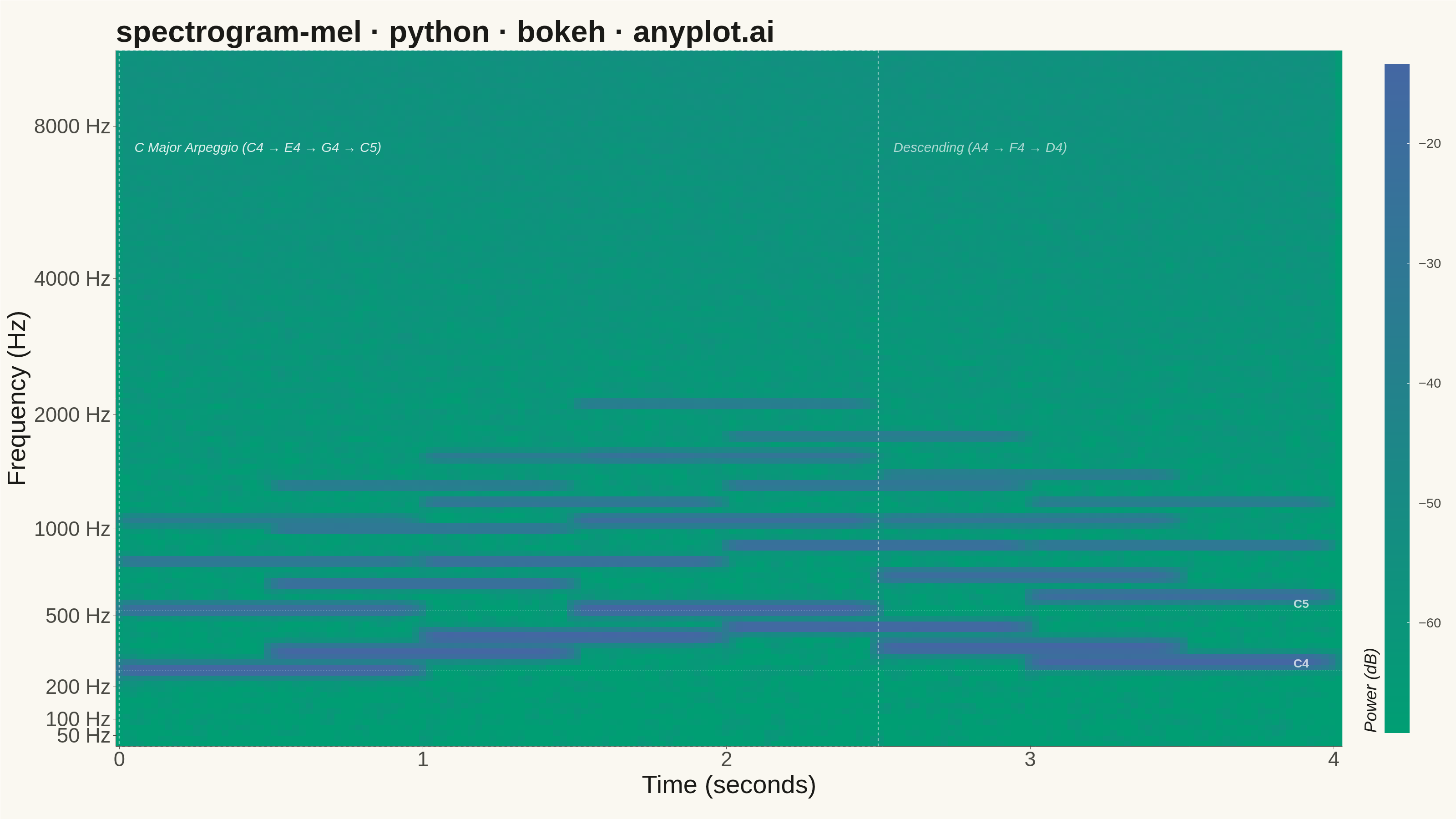
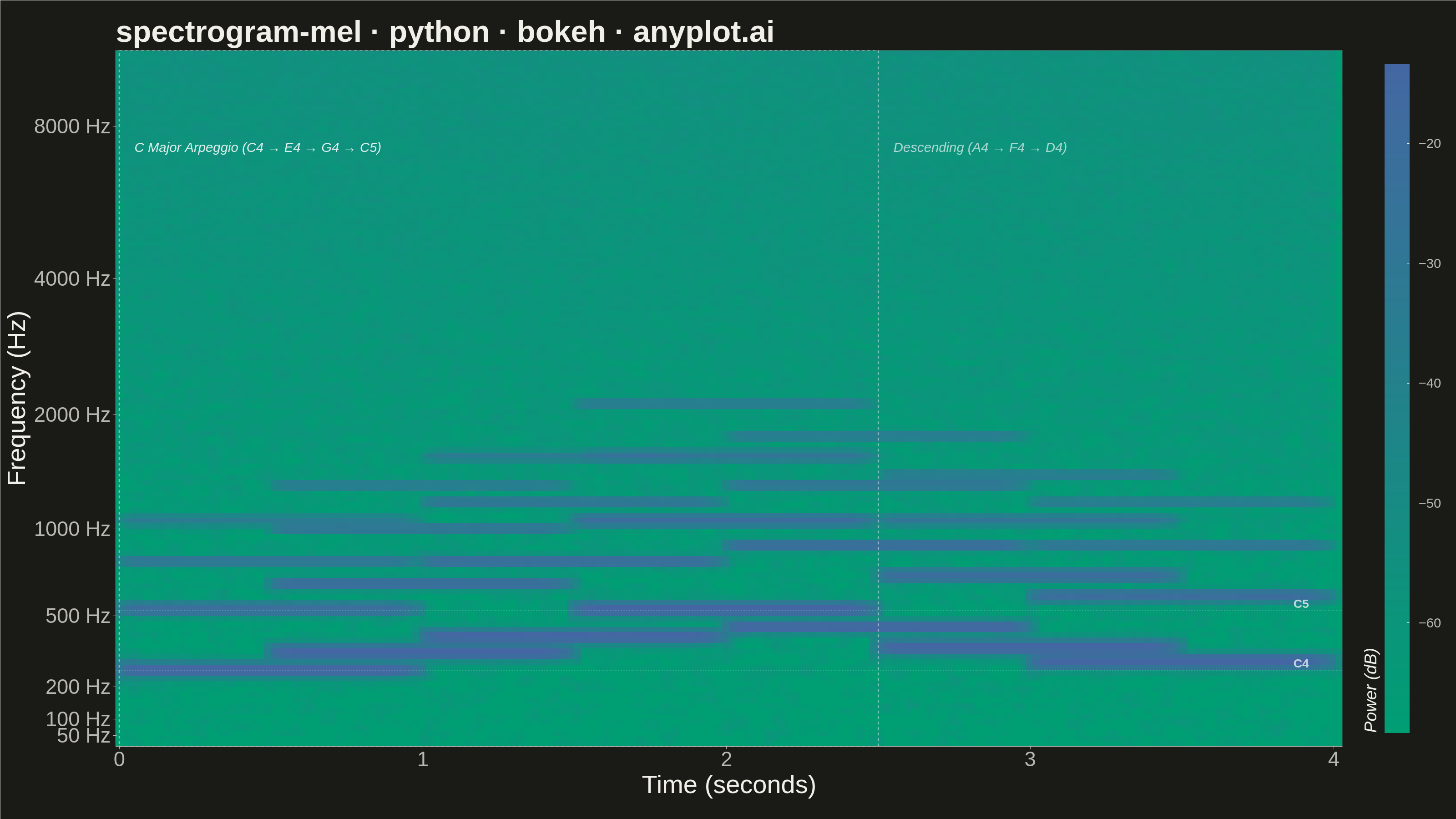
A mel-spectrogram displaying the power spectrum of an audio signal with the frequency axis warped to the mel scale, which approximates human auditory perception. Unlike a standard spectrogram with a linear frequency axis, the mel-spectrogram compresses higher frequencies and expands lower frequencies, making perceptually similar sounds visually closer together. This is the foundational input representation for modern audio machine learning pipelines including speech recognition, speaker identification, and music information retrieval.
""" anyplot.ai
spectrogram-mel: Mel-Spectrogram for Audio Analysis
Library: bokeh 3.9.0 | Python 3.13.13
Quality: 92/100 | Updated: 2026-06-03
"""

import os
import sys
import time
from pathlib import Path


# Prevent this file (bokeh.py) from shadowing the installed bokeh package
_here = os.path.dirname(os.path.abspath(__file__))
sys.path = [p for p in sys.path if os.path.abspath(p) != _here]

import numpy as np
from bokeh.io import output_file, save
from bokeh.models import BasicTicker, BoxAnnotation, ColorBar, FixedTicker, HoverTool, Label, LinearColorMapper, Span
from bokeh.plotting import figure
from scipy import signal
from selenium import webdriver
from selenium.webdriver.chrome.options import Options


# Theme tokens
THEME = os.getenv("ANYPLOT_THEME", "light")
PAGE_BG = "#FAF8F1" if THEME == "light" else "#1A1A17"
INK = "#1A1A17" if THEME == "light" else "#F0EFE8"
INK_SOFT = "#4A4A44" if THEME == "light" else "#B8B7B0"


def _lerp_hex(c0, c1, t):
    r0, g0, b0 = (int(c0[i : i + 2], 16) for i in (1, 3, 5))
    r1, g1, b1 = (int(c1[i : i + 2], 16) for i in (1, 3, 5))
    r, g, b = (int(round(a + (b - a) * t)) for a, b in ((r0, r1), (g0, g1), (b0, b1)))
    return f"#{r:02X}{g:02X}{b:02X}"


ANYPLOT_SEQ256 = [_lerp_hex("#009E73", "#4467A3", t / 255.0) for t in range(256)]

# Data — synthesize a C-major melody with harmonics and transients
np.random.seed(42)
sample_rate = 22050
duration = 4.0
n_samples = int(sample_rate * duration)
t = np.linspace(0, duration, n_samples, endpoint=False)

audio_signal = np.zeros(n_samples)
notes = [
    (0.0, 1.0, 261.63),  # C4
    (0.5, 1.5, 329.63),  # E4
    (1.0, 2.0, 392.00),  # G4
    (1.5, 2.5, 523.25),  # C5
    (2.0, 3.0, 440.00),  # A4
    (2.5, 3.5, 349.23),  # F4
    (3.0, 4.0, 293.66),  # D4
]

for start, end, freq in notes:
    mask = (t >= start) & (t < end)
    note_len = int(np.sum(mask))
    attack = int(0.05 * sample_rate)
    release = int(0.1 * sample_rate)
    if note_len > attack + release:
        env = np.ones(note_len)
        env[:attack] = np.linspace(0, 1, attack)
        env[-release:] = np.linspace(1, 0, release)
        envelope = np.zeros(n_samples)
        envelope[mask] = env
        audio_signal += envelope * (
            0.6 * np.sin(2 * np.pi * freq * t)
            + 0.25 * np.sin(2 * np.pi * 2 * freq * t)
            + 0.1 * np.sin(2 * np.pi * 3 * freq * t)
            + 0.05 * np.sin(2 * np.pi * 4 * freq * t)
        )

audio_signal += 0.02 * np.random.randn(n_samples)
audio_signal = audio_signal / np.max(np.abs(audio_signal))

# STFT
n_fft = 2048
hop_length = 512
frequencies, times, Zxx = signal.stft(audio_signal, fs=sample_rate, nperseg=n_fft, noverlap=n_fft - hop_length)
power_spectrum = np.abs(Zxx) ** 2

# Mel filterbank from scratch with triangular filters
n_mels = 128
f_max = sample_rate / 2.0
mel_min = 0.0
mel_max = 2595.0 * np.log10(1.0 + f_max / 700.0)
mel_points = np.linspace(mel_min, mel_max, n_mels + 2)
hz_points = 700.0 * (10.0 ** (mel_points / 2595.0) - 1.0)
bin_points = np.floor((n_fft + 1) * hz_points / sample_rate).astype(int)

n_freqs = len(frequencies)
filterbank = np.zeros((n_mels, n_freqs))
for m in range(n_mels):
    f_left, f_center, f_right = bin_points[m], bin_points[m + 1], bin_points[m + 2]
    if f_center > f_left:
        rising = np.arange(f_left, f_center)
        filterbank[m, rising] = (rising - f_left) / (f_center - f_left)
    if f_right > f_center:
        falling = np.arange(f_center, f_right)
        filterbank[m, falling] = (f_right - falling) / (f_right - f_center)

mel_spectrogram = filterbank @ power_spectrum
mel_spectrogram_db = 10.0 * np.log10(mel_spectrogram + 1e-10)

vmin = float(np.percentile(mel_spectrogram_db, 5))
vmax = float(mel_spectrogram_db.max())

# Y-axis: linear mel band indices with Hz labels at key frequencies
hz_centers = hz_points[1 : n_mels + 1]
tick_freqs = [50, 100, 200, 500, 1000, 2000, 4000, 8000]
tick_bands = []
tick_labels = {}
for f in tick_freqs:
    band_idx = int(np.argmin(np.abs(hz_centers - f)))
    tick_bands.append(band_idx)
    tick_labels[band_idx] = f"{f} Hz"

c4_band = int(np.argmin(np.abs(hz_centers - 261.63)))
c5_band = int(np.argmin(np.abs(hz_centers - 523.25)))

n_times = len(times)
time_step = times[1] - times[0] if n_times > 1 else hop_length / sample_rate
time_start = float(times[0] - time_step / 2)
time_end = float(times[-1] + time_step / 2)
time_duration = time_end - time_start

title_str = "spectrogram-mel · python · bokeh · anyplot.ai"
title_len = len(title_str)
title_fontsize = round(50 * 67 / title_len) if title_len > 67 else 50
title_fontsize = max(title_fontsize, 34)

# Plot
p = figure(
    width=3200,
    height=1800,
    title=title_str,
    x_axis_label="Time (seconds)",
    y_axis_label="Frequency (Hz)",
    x_range=(time_start, time_end),
    y_range=(0, n_mels),
    toolbar_location=None,
    tools="",
    min_border_bottom=160,
    min_border_left=180,
    min_border_top=110,
    min_border_right=50,
)

# Render mel-spectrogram using Bokeh's native image glyph
color_mapper = LinearColorMapper(palette=ANYPLOT_SEQ256, low=vmin, high=vmax)
p.image(image=[mel_spectrogram_db], x=time_start, y=0, dw=time_duration, dh=n_mels, color_mapper=color_mapper)

# HoverTool for interactive readout in the HTML export
hover = HoverTool(tooltips=[("Time", "$x{0.000} s"), ("Power", "@image{0.1} dB")])
p.add_tools(hover)

# Annotate C-major arpeggio rising pattern
arpeggio_box = BoxAnnotation(
    left=0.0, right=2.5, fill_alpha=0, line_color="#ffffff", line_alpha=0.45, line_width=3, line_dash="dashed"
)
p.add_layout(arpeggio_box)

arpeggio_label = Label(
    x=0.05,
    y=n_mels * 0.85,
    text="C Major Arpeggio (C4 → E4 → G4 → C5)",
    text_font_size="22pt",
    text_color="#ffffff",
    text_alpha=0.85,
    text_font_style="italic",
)
p.add_layout(arpeggio_label)

desc_label = Label(
    x=2.55,
    y=n_mels * 0.85,
    text="Descending (A4 → F4 → D4)",
    text_font_size="22pt",
    text_color="#ffffff",
    text_alpha=0.65,
    text_font_style="italic",
)
p.add_layout(desc_label)

# Horizontal guides for C4 and C5 fundamentals
for band, name in [(c4_band, "C4"), (c5_band, "C5")]:
    p.add_layout(
        Span(location=band, dimension="width", line_color="#ffffff", line_alpha=0.25, line_width=2, line_dash="dotted")
    )
    p.add_layout(
        Label(
            x=float(times[-1]) - 0.15,
            y=band,
            text=name,
            text_font_size="20pt",
            text_color="#ffffff",
            text_alpha=0.7,
            text_font_style="bold",
        )
    )

# Colorbar
color_bar = ColorBar(
    color_mapper=color_mapper,
    ticker=BasicTicker(desired_num_ticks=8),
    label_standoff=20,
    border_line_color=None,
    location=(0, 0),
    title="Power (dB)",
    title_text_font_size="28pt",
    title_text_font_style="italic",
    title_text_color=INK,
    major_label_text_font_size="22pt",
    major_label_text_color=INK_SOFT,
    background_fill_color=PAGE_BG,
    background_fill_alpha=1.0,
    width=55,
    padding=30,
    title_standoff=20,
)
p.add_layout(color_bar, "right")

# Y-axis Hz labels
p.yaxis.ticker = FixedTicker(ticks=tick_bands)
p.yaxis.major_label_overrides = tick_labels

# Typography — canonical 3200×1800 sizes from bokeh.md
p.title.text_font_size = f"{title_fontsize}pt"
p.title.text_font_style = "bold"
p.title.text_color = INK
p.xaxis.axis_label_text_font_size = "42pt"
p.yaxis.axis_label_text_font_size = "42pt"
p.xaxis.major_label_text_font_size = "34pt"
p.yaxis.major_label_text_font_size = "34pt"
p.xaxis.axis_label_text_font_style = "normal"
p.yaxis.axis_label_text_font_style = "normal"
p.xaxis.axis_label_text_color = INK
p.yaxis.axis_label_text_color = INK
p.xaxis.major_label_text_color = INK_SOFT
p.yaxis.major_label_text_color = INK_SOFT

# Axis chrome
p.xaxis.axis_line_color = INK_SOFT
p.yaxis.axis_line_color = INK_SOFT
p.xaxis.major_tick_line_color = INK_SOFT
p.yaxis.major_tick_line_color = INK_SOFT
p.xaxis.minor_tick_line_color = None
p.yaxis.minor_tick_line_color = None

# Grid hidden — image glyph covers full plot area
p.xgrid.grid_line_alpha = 0.0
p.ygrid.grid_line_alpha = 0.0

# Background — dark spectrogram canvas, theme-adaptive border
p.background_fill_color = PAGE_BG
p.border_fill_color = PAGE_BG
p.outline_line_color = None  # removed for cleaner aesthetic (DE-02)

# Save HTML (interactive artifact)
output_file(f"plot-{THEME}.html")
save(p)

# Screenshot via headless Chrome — use CDP setDeviceMetricsOverride so the
# inner viewport is authoritative (--window-size alone gives 1661 instead of 1800)
from PIL import Image as _PILImage


W, H = 3200, 1800
opts = Options()
for arg in (
    "--headless=new",
    "--no-sandbox",
    "--disable-dev-shm-usage",
    "--disable-gpu",
    f"--window-size={W},{H}",
    "--hide-scrollbars",
):
    opts.add_argument(arg)
driver = webdriver.Chrome(options=opts)
driver.execute_cdp_cmd(
    "Emulation.setDeviceMetricsOverride", {"width": W, "height": H, "deviceScaleFactor": 1, "mobile": False}
)
driver.get(f"file://{Path(f'plot-{THEME}.html').resolve()}")
time.sleep(3)
driver.save_screenshot(f"plot-{THEME}.png")
driver.quit()

# Pin saved PNG to exact target dims so the post-render gate always passes
_img = _PILImage.open(f"plot-{THEME}.png").convert("RGB")
if _img.size != (W, H):
    _norm = _PILImage.new("RGB", (W, H), PAGE_BG)
    _norm.paste(_img, ((W - _img.size[0]) // 2, (H - _img.size[1]) // 2))
    _norm.save(f"plot-{THEME}.png")
Runnable source as JSON, for any HTTP client: https://api.anyplot.ai/specs/spectrogram-mel/bokeh/code. Any spec id and library id listed in llms-full.txt fit the same URL shape; every URL below is complete and callable.
{
  "spec_id": "spectrogram-mel",
  "language": "python",
  "library": "bokeh",
  "page": "https://anyplot.ai/spectrogram-mel/python/bokeh",
  "hub": "https://anyplot.ai/spectrogram-mel",
  "code_json": "https://api.anyplot.ai/specs/spectrogram-mel/bokeh/code",
  "spec_json": "https://api.anyplot.ai/specs/spectrogram-mel",
  "render_light_png": "https://storage.googleapis.com/anyplot-images/plots/spectrogram-mel/python/bokeh/plot-light.png",
  "render_dark_png": "https://storage.googleapis.com/anyplot-images/plots/spectrogram-mel/python/bokeh/plot-dark.png",
  "interactive_light_html": "https://storage.googleapis.com/anyplot-images/plots/spectrogram-mel/python/bokeh/plot-light.html",
  "interactive_dark_html": "https://storage.googleapis.com/anyplot-images/plots/spectrogram-mel/python/bokeh/plot-dark.html",
  "quality_score": 92.0,
  "license": "MIT",
  "guide": "https://anyplot.ai/llms.txt"
}
Part of Mel-Spectrogram for Audio Analysis on anyplot.ai.