The same plot in 14 other libraries — Python: Altair, Bokeh, lets-plot, Matplotlib, Plotly, plotnine, Pygal, Seaborn; Julia: Makie.jl; JavaScript: Chart.js, D3.js, Apache ECharts, Highcharts, MUI X Charts. Compare all 15 side by side: Mel-Spectrogram for Audio Analysis in Python, R, Julia and JavaScript.
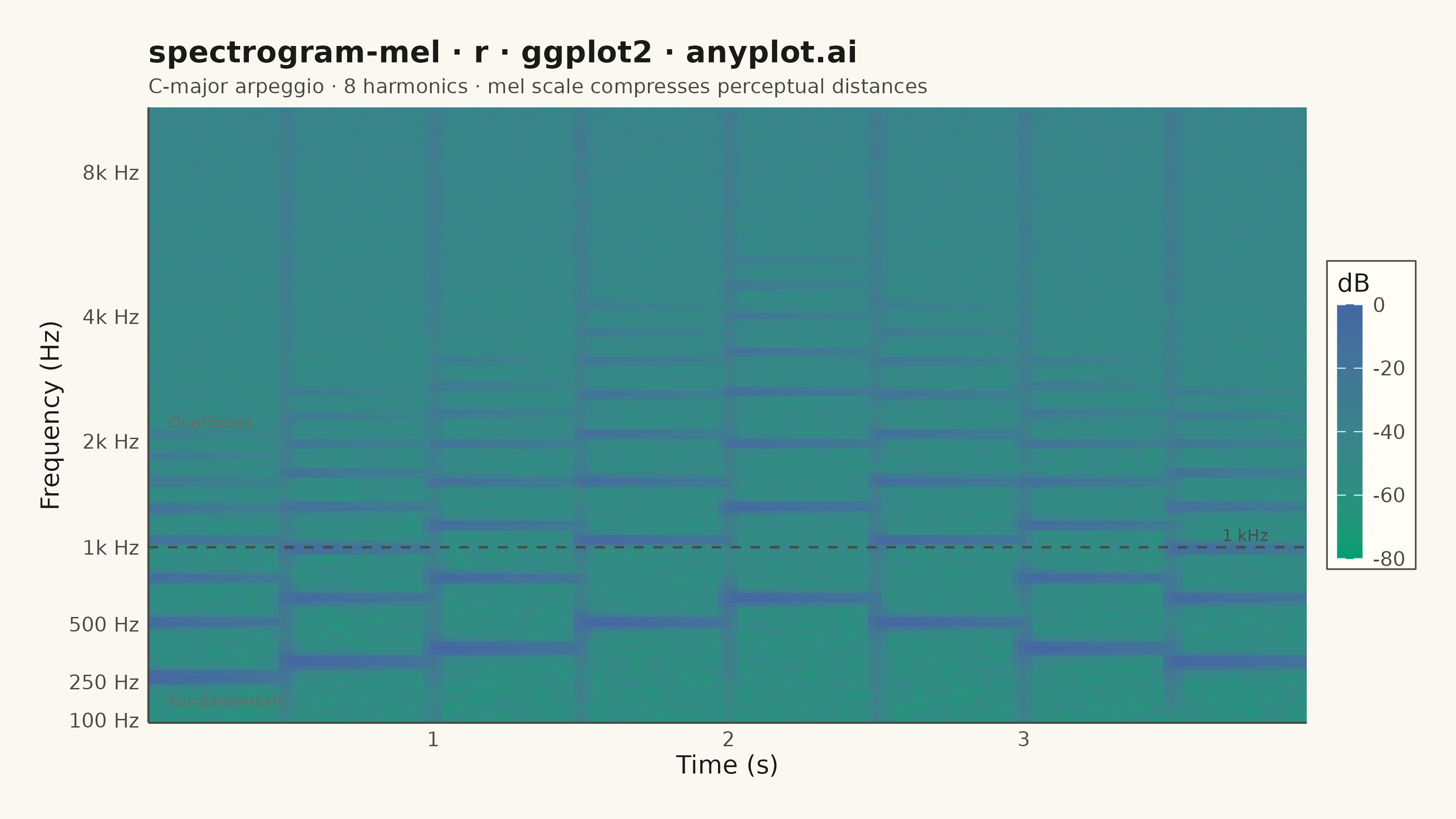
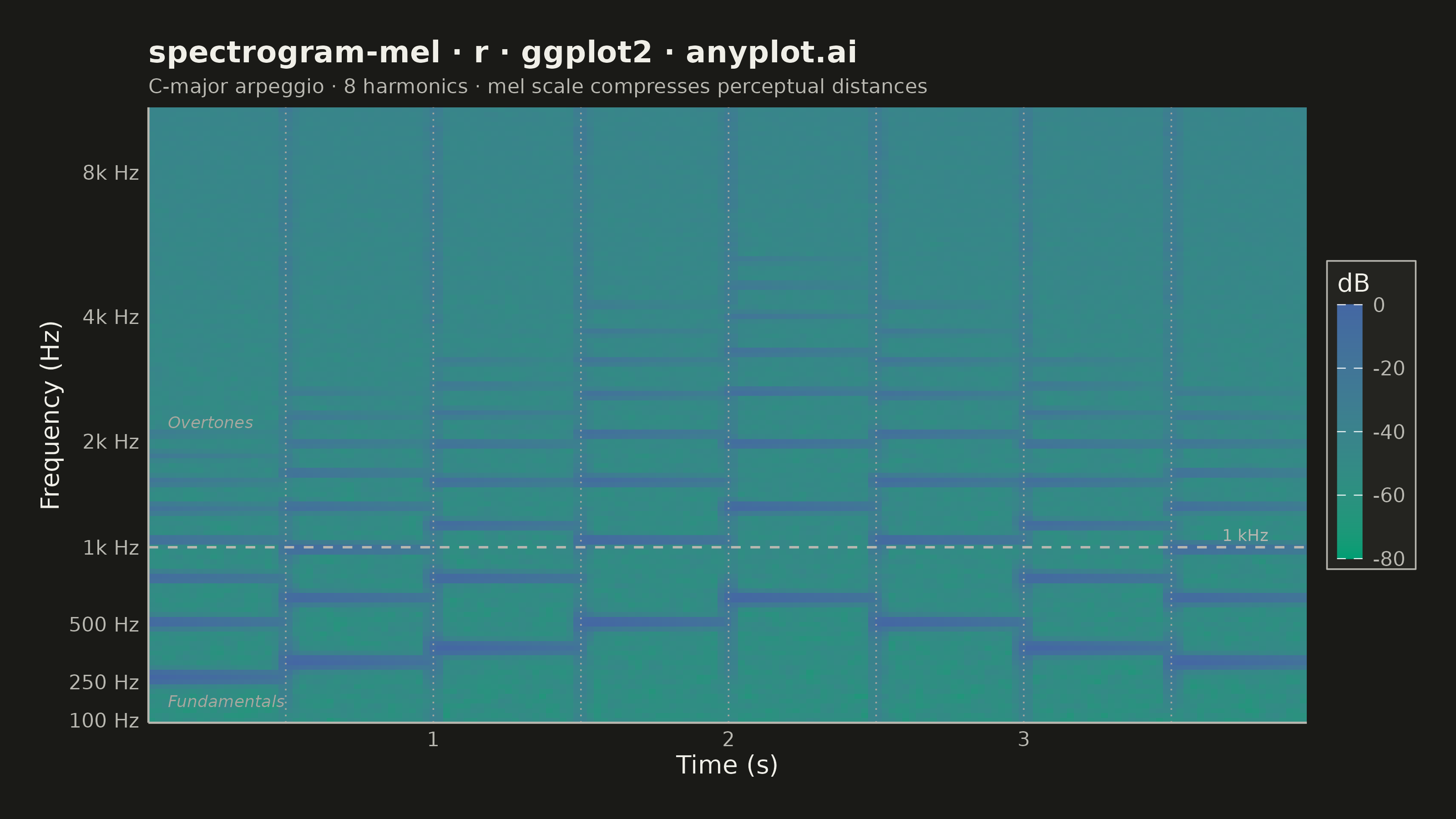
A mel-spectrogram displaying the power spectrum of an audio signal with the frequency axis warped to the mel scale, which approximates human auditory perception. Unlike a standard spectrogram with a linear frequency axis, the mel-spectrogram compresses higher frequencies and expands lower frequencies, making perceptually similar sounds visually closer together. This is the foundational input representation for modern audio machine learning pipelines including speech recognition, speaker identification, and music information retrieval.
#' anyplot.ai
#' spectrogram-mel: Mel-Spectrogram for Audio Analysis
#' Library: ggplot2 3.5.1 | R 4.4.1
#' Quality: 88/100 | Created: 2026-06-03

library(ggplot2)
library(scales)
library(ragg)

set.seed(42)

# --- Theme tokens ---
THEME       <- Sys.getenv("ANYPLOT_THEME", "light")
PAGE_BG     <- if (THEME == "light") "#FAF8F1" else "#1A1A17"
ELEVATED_BG <- if (THEME == "light") "#FFFDF6" else "#242420"
INK         <- if (THEME == "light") "#1A1A17" else "#F0EFE8"
INK_SOFT    <- if (THEME == "light") "#4A4A44" else "#B8B7B0"
INK_MUTED   <- if (THEME == "light") "#6B6A63" else "#A8A79F"

# --- Audio parameters ---
sample_rate <- 22050L
duration    <- 4.0
n_fft       <- 2048L
hop_length  <- 512L
n_mels      <- 128L

# --- Synthesize audio: C-major arpeggio with 8 harmonics + percussive transients ---
n_samples  <- as.integer(sample_rate * duration)
t_vec      <- seq(0, duration, length.out = n_samples + 1L)[seq_len(n_samples)]
note_freqs <- c(261.63, 329.63, 392.00, 523.25, 659.25, 523.25, 392.00, 329.63)
note_dur   <- duration / length(note_freqs)

audio    <- numeric(n_samples)
harm_amp <- 0.5 * 0.6^(0:7)  # 8 harmonics with exponential amplitude decay

for (i in seq_along(note_freqs)) {
  t0  <- (i - 1L) * note_dur
  idx <- which(t_vec >= t0 & t_vec < t0 + note_dur)
  f   <- note_freqs[i]
  dt  <- t_vec[idx] - t0
  env <- pmax(0, (1 - exp(-300 * dt)) * exp(-4 * dt))
  wave <- Reduce("+", lapply(seq_along(harm_amp), function(h) {
    harm_amp[h] * sin(2 * pi * h * f * t_vec[idx])
  }))
  # Percussive onset burst: broadband noise decaying over ~25 ms
  burst_len <- min(as.integer(0.025 * sample_rate), length(idx))
  burst_env <- c(exp(-150 * dt[seq_len(burst_len)]), numeric(length(idx) - burst_len))
  audio[idx] <- env * wave + 0.18 * burst_env * rnorm(length(idx))
}
audio <- audio + 0.012 * rnorm(n_samples)

# --- STFT: Hann-windowed power spectrogram ---
n_fft_half <- n_fft %/% 2L + 1L
hann_win   <- 0.5 * (1 - cos(2 * pi * seq(0L, n_fft - 1L) / (n_fft - 1L)))
n_frames   <- floor((n_samples - n_fft) / hop_length) + 1L

stft_power <- matrix(0.0, nrow = n_fft_half, ncol = n_frames)
for (i in seq_len(n_frames)) {
  s <- (i - 1L) * hop_length + 1L
  stft_power[, i] <- Mod(fft(audio[s:(s + n_fft - 1L)] * hann_win)[seq_len(n_fft_half)])^2
}

# --- Mel filterbank ---
hz_to_mel <- function(f) 2595 * log10(1 + f / 700)
mel_to_hz <- function(m) 700 * (10^(m / 2595) - 1)

f_min     <- 80.0
f_max     <- as.numeric(sample_rate) / 2.0
mel_pts   <- seq(hz_to_mel(f_min), hz_to_mel(f_max), length.out = n_mels + 2L)
hz_pts    <- mel_to_hz(mel_pts)
fft_freqs <- seq(0, f_max, length.out = n_fft_half)

mel_fb <- matrix(0.0, nrow = n_mels, ncol = n_fft_half)
for (m in seq_len(n_mels)) {
  rising  <- (fft_freqs - hz_pts[m])      / (hz_pts[m + 1L] - hz_pts[m])
  falling <- (hz_pts[m + 2L] - fft_freqs) / (hz_pts[m + 2L] - hz_pts[m + 1L])
  mel_fb[m, ] <- pmax(0.0, pmin(rising, falling))
}

# --- Mel spectrogram in dB, normalized to 0 dB peak ---
mel_spec    <- mel_fb %*% stft_power
mel_spec_db <- 10 * log10(mel_spec + 1e-10)
mel_spec_db <- mel_spec_db - max(mel_spec_db)

# --- Long-format data frame ---
mel_centers <- mel_to_hz(mel_pts[2:(n_mels + 1L)])
time_axis   <- ((seq_len(n_frames) - 1L) * hop_length + n_fft / 2L) / sample_rate

grid_idx <- expand.grid(mel_band = seq_len(n_mels), time_idx = seq_len(n_frames))
df <- data.frame(
  time_s   = time_axis[grid_idx$time_idx],
  mel_band = grid_idx$mel_band,
  db       = mel_spec_db[cbind(grid_idx$mel_band, grid_idx$time_idx)]
)

# Y-axis: key frequency labels at representative mel-band positions
key_freqs  <- c(100, 250, 500, 1000, 2000, 4000, 8000)
key_bands  <- sapply(key_freqs, function(f) which.min(abs(mel_centers - f)))
key_labels <- ifelse(key_freqs >= 1000, paste0(key_freqs / 1000, "k Hz"), paste0(key_freqs, " Hz"))

# Annotation reference positions
note_onsets <- (seq_along(note_freqs) - 1L) * note_dur
band_1k     <- which.min(abs(mel_centers - 1000))
band_2k     <- which.min(abs(mel_centers - 2000))
t_max       <- max(time_axis)

title_str <- "spectrogram-mel · r · ggplot2 · anyplot.ai"

# --- Plot ---
p <- ggplot(df, aes(x = time_s, y = mel_band, fill = db)) +
  geom_tile() +
  # Note onset markers — reveal rhythmic structure of the arpeggio
  geom_vline(
    xintercept = note_onsets[-1],
    color      = INK_MUTED,
    linewidth  = 0.3,
    linetype   = "dotted"
  ) +
  # Perceptual boundary: 1 kHz separates fundamental region from overtones
  geom_hline(
    yintercept = band_1k,
    color      = INK_SOFT,
    linewidth  = 0.45,
    linetype   = "dashed"
  ) +
  annotate("text",
    x = t_max * 0.97, y = band_1k + 2.5,
    label = "1 kHz", color = INK_SOFT,
    size = 2.3, hjust = 1
  ) +
  # Frequency region labels for interpretive guidance
  annotate("text",
    x = 0.10, y = 5,
    label = "Fundamentals", color = INK_MUTED,
    size = 2.3, hjust = 0, fontface = "italic"
  ) +
  annotate("text",
    x = 0.10, y = band_2k + 4,
    label = "Overtones", color = INK_MUTED,
    size = 2.3, hjust = 0, fontface = "italic"
  ) +
  scale_fill_gradient(
    name   = "dB",
    low    = "#009E73",
    high   = "#4467A3",
    limits = c(-80, 0),
    oob    = scales::squish,
    breaks = c(0, -20, -40, -60, -80)
  ) +
  scale_x_continuous(
    name   = "Time (s)",
    expand = c(0, 0)
  ) +
  scale_y_continuous(
    name   = "Frequency (Hz)",
    breaks = key_bands,
    labels = key_labels,
    expand = c(0, 0)
  ) +
  guides(fill = guide_colorbar(barheight = 7, barwidth = 0.7, ticks = TRUE)) +
  labs(
    title    = title_str,
    subtitle = "C-major arpeggio · 8 harmonics · mel scale compresses perceptual distances"
  ) +
  theme_minimal(base_size = 8) +
  theme(
    plot.background   = element_rect(fill = PAGE_BG,     color = PAGE_BG),
    panel.background  = element_rect(fill = PAGE_BG,     color = NA),
    panel.grid.major  = element_blank(),
    panel.grid.minor  = element_blank(),
    panel.border      = element_blank(),
    axis.title        = element_text(color = INK,        size = 10),
    axis.text         = element_text(color = INK_SOFT,   size = 8),
    axis.line         = element_line(color = INK_SOFT,   linewidth = 0.4),
    plot.title        = element_text(color = INK,        size = 12, face = "bold"),
    plot.subtitle     = element_text(color = INK_SOFT,   size = 8),
    legend.background = element_rect(fill = ELEVATED_BG, color = INK_SOFT, linewidth = 0.3),
    legend.text       = element_text(color = INK_SOFT,   size = 8),
    legend.title      = element_text(color = INK,        size = 10),
    plot.margin       = margin(16, 16, 16, 16)
  )

# --- Save ---
ggsave(
  filename = sprintf("plot-%s.png", THEME),
  plot     = p,
  device   = ragg::agg_png,
  width    = 8,
  height   = 4.5,
  units    = "in",
  dpi      = 400
)
Runnable source as JSON, for any HTTP client: https://api.anyplot.ai/specs/spectrogram-mel/ggplot2/code. Any spec id and library id listed in llms-full.txt fit the same URL shape; every URL below is complete and callable.
{
  "spec_id": "spectrogram-mel",
  "language": "r",
  "library": "ggplot2",
  "page": "https://anyplot.ai/spectrogram-mel/r/ggplot2",
  "hub": "https://anyplot.ai/spectrogram-mel",
  "code_json": "https://api.anyplot.ai/specs/spectrogram-mel/ggplot2/code",
  "spec_json": "https://api.anyplot.ai/specs/spectrogram-mel",
  "render_light_png": "https://storage.googleapis.com/anyplot-images/plots/spectrogram-mel/r/ggplot2/plot-light.png",
  "render_dark_png": "https://storage.googleapis.com/anyplot-images/plots/spectrogram-mel/r/ggplot2/plot-dark.png",
  "quality_score": 88.0,
  "license": "MIT",
  "guide": "https://anyplot.ai/llms.txt"
}
Part of Mel-Spectrogram for Audio Analysis on anyplot.ai.