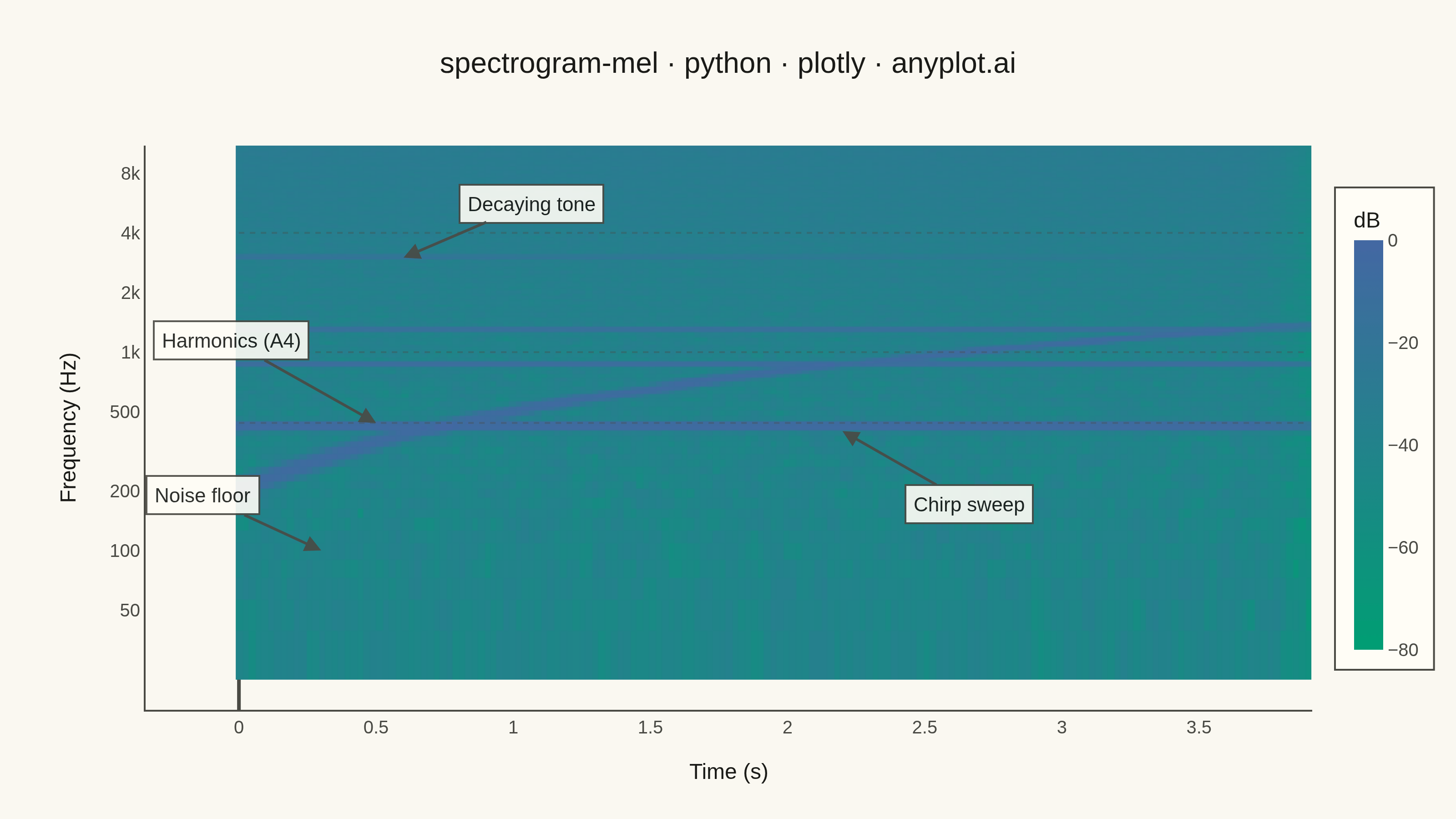
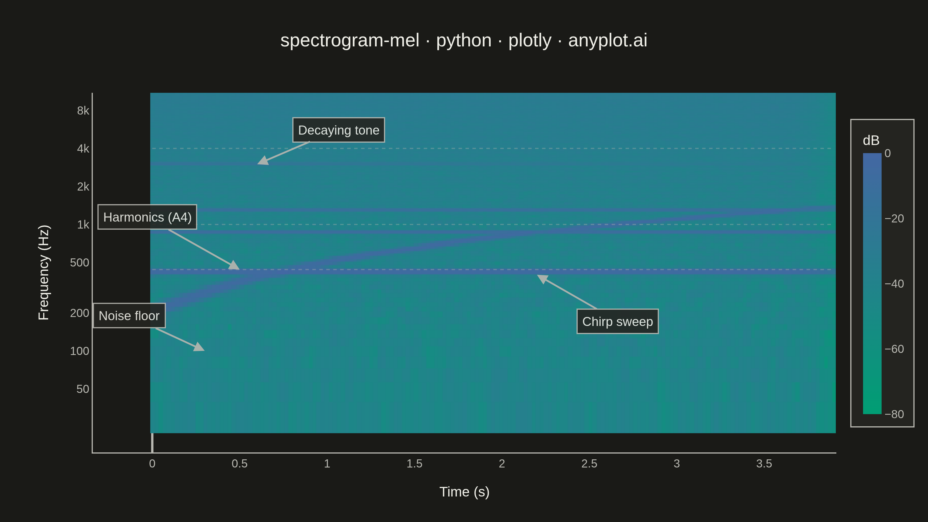
A mel-spectrogram displaying the power spectrum of an audio signal with the frequency axis warped to the mel scale, which approximates human auditory perception. Unlike a standard spectrogram with a linear frequency axis, the mel-spectrogram compresses higher frequencies and expands lower frequencies, making perceptually similar sounds visually closer together. This is the foundational input representation for modern audio machine learning pipelines including speech recognition, speaker identification, and music information retrieval.
""" anyplot.ai
spectrogram-mel: Mel-Spectrogram for Audio Analysis
Library: plotly 6.7.0 | Python 3.13.13
Quality: 90/100 | Updated: 2026-06-03
"""

import os

import numpy as np
import plotly.graph_objects as go


# Theme-adaptive chrome — Imprint palette
THEME = os.getenv("ANYPLOT_THEME", "light")
PAGE_BG = "#FAF8F1" if THEME == "light" else "#1A1A17"
ELEVATED_BG = "#FFFDF6" if THEME == "light" else "#242420"
INK = "#1A1A17" if THEME == "light" else "#F0EFE8"
INK_SOFT = "#4A4A44" if THEME == "light" else "#B8B7B0"

# Imprint sequential colormap for single-polarity continuous data (dB magnitude)
imprint_seq = [[0.0, "#009E73"], [1.0, "#4467A3"]]

# Reference line color — theme-adaptive subtle overlay
REF_COLOR = "rgba(74,74,68,0.35)" if THEME == "light" else "rgba(184,183,176,0.35)"

# Data: synthesize audio with melody-like frequency components
np.random.seed(42)
sample_rate = 22050
duration = 4.0
n_samples = int(sample_rate * duration)
t = np.linspace(0, duration, n_samples, endpoint=False)

signal = (
    0.5 * np.sin(2 * np.pi * 440 * t)
    + 0.3 * np.sin(2 * np.pi * 880 * t)
    + 0.2 * np.sin(2 * np.pi * 1320 * t)
    + 0.4 * np.sin(2 * np.pi * (200 + 600 * t / duration) * t)
    + 0.15 * np.sin(2 * np.pi * 3000 * t) * np.exp(-t / 2)
    + 0.1 * np.random.randn(n_samples)
)
# Amplitude envelope: short fade-in, extended fade-out
envelope = np.ones(n_samples)
envelope[: int(0.05 * sample_rate)] = np.linspace(0, 1, int(0.05 * sample_rate))
envelope[-int(0.3 * sample_rate) :] = np.linspace(1, 0, int(0.3 * sample_rate))
signal *= envelope

# STFT computation (manual, no librosa dependency)
n_fft = 2048
hop_length = 512
window = np.hanning(n_fft)
n_frames = 1 + (n_samples - n_fft) // hop_length
stft_matrix = np.zeros((n_fft // 2 + 1, n_frames))
for i in range(n_frames):
    start = i * hop_length
    frame = signal[start : start + n_fft] * window
    stft_matrix[:, i] = np.abs(np.fft.rfft(frame)) ** 2

# Mel filterbank construction
n_mels = 128
f_min, f_max = 0.0, sample_rate / 2.0
mel_min = 2595.0 * np.log10(1.0 + f_min / 700.0)
mel_max = 2595.0 * np.log10(1.0 + f_max / 700.0)
mel_points = np.linspace(mel_min, mel_max, n_mels + 2)
hz_points = 700.0 * (10.0 ** (mel_points / 2595.0) - 1.0)
freq_bins = np.floor((n_fft + 1) * hz_points / sample_rate).astype(int)

filterbank = np.zeros((n_mels, n_fft // 2 + 1))
for m in range(1, n_mels + 1):
    f_left, f_center, f_right = freq_bins[m - 1], freq_bins[m], freq_bins[m + 1]
    for k in range(f_left, f_center):
        if f_center != f_left:
            filterbank[m - 1, k] = (k - f_left) / (f_center - f_left)
    for k in range(f_center, f_right):
        if f_right != f_center:
            filterbank[m - 1, k] = (f_right - k) / (f_right - f_center)

# Mel spectrogram in dB (normalised to 0 dB peak)
mel_spec = filterbank @ stft_matrix
mel_spec = np.maximum(mel_spec, 1e-10)
mel_spec_db = 10.0 * np.log10(mel_spec) - 10.0 * np.log10(mel_spec.max())

# Time and frequency axes
time_axis = np.arange(n_frames) * hop_length / sample_rate
mel_freq_points = np.linspace(mel_min, mel_max, n_mels)
mel_freqs = 700.0 * (10.0 ** (mel_freq_points / 2595.0) - 1.0)

# Plot
fig = go.Figure(
    data=go.Heatmap(
        z=mel_spec_db,
        x=time_axis,
        y=mel_freqs,
        colorscale=imprint_seq,
        colorbar={
            "title": {"text": "dB", "font": {"size": 12, "color": INK}},
            "tickfont": {"size": 10, "color": INK_SOFT},
            "thickness": 16,
            "len": 0.85,
            "bgcolor": ELEVATED_BG,
            "bordercolor": INK_SOFT,
            "borderwidth": 1,
        },
        zmin=-80,
        zmax=0,
        hovertemplate="Time: %{x:.2f}s<br>Freq: %{y:.0f} Hz<br>Power: %{z:.1f} dB<extra></extra>",
    )
)

fig.update_layout(
    autosize=False,
    paper_bgcolor=PAGE_BG,
    plot_bgcolor=PAGE_BG,
    font={"color": INK},
    title={
        "text": "spectrogram-mel · python · plotly · anyplot.ai", "font": {"size": 16, "color": INK}, "x": 0.5, "xanchor": "center"
    },
    xaxis={
        "title": {"text": "Time (s)", "font": {"size": 12, "color": INK}},
        "tickfont": {"size": 10, "color": INK_SOFT},
        "showgrid": False,
        "linecolor": INK_SOFT,
        "zerolinecolor": INK_SOFT,
    },
    yaxis={
        "title": {"text": "Frequency (Hz)", "font": {"size": 12, "color": INK}},
        "tickfont": {"size": 10, "color": INK_SOFT},
        "type": "log",
        "tickvals": [50, 100, 200, 500, 1000, 2000, 4000, 8000],
        "ticktext": ["50", "100", "200", "500", "1k", "2k", "4k", "8k"],
        "showgrid": False,
        "linecolor": INK_SOFT,
        "zerolinecolor": INK_SOFT,
        "range": [np.log10(mel_freqs[1]), np.log10(mel_freqs[-1])],
    },
    margin={"l": 80, "r": 40, "t": 80, "b": 60},
    hoverlabel={"bgcolor": ELEVATED_BG, "font_size": 10, "font_family": "monospace", "font_color": INK, "bordercolor": INK_SOFT},
)

# Subtle reference lines at perceptually meaningful frequency bands
for freq in [440, 1000, 4000]:
    fig.add_shape(
        type="line",
        x0=time_axis[0],
        x1=time_axis[-1],
        y0=freq,
        y1=freq,
        line={"color": REF_COLOR, "width": 1, "dash": "dot"},
    )

# Annotations guiding viewer through key spectral features
for ann in [
    {"x": 0.5, "y": np.log10(440), "text": "Harmonics (A4)", "ax": -80, "ay": -45},
    {"x": 2.2, "y": np.log10(400), "text": "Chirp sweep", "ax": 70, "ay": 40},
    {"x": 0.6, "y": np.log10(3000), "text": "Decaying tone", "ax": 70, "ay": -30},
    {"x": 0.3, "y": np.log10(100), "text": "Noise floor", "ax": -65, "ay": -30},
]:
    fig.add_annotation(
        x=ann["x"],
        y=ann["y"],
        yref="y",
        text=ann["text"],
        showarrow=True,
        arrowhead=2,
        arrowsize=1.2,
        arrowwidth=1.5,
        arrowcolor=INK_SOFT,
        ax=ann["ax"],
        ay=ann["ay"],
        font={"size": 11, "color": INK, "family": "Arial"},
        bordercolor=INK_SOFT,
        borderwidth=1,
        borderpad=4,
        bgcolor=ELEVATED_BG,
        opacity=0.9,
    )

# Save — canvas: 800×450 × scale=4 → 3200×1800 px (landscape)
fig.write_image(f"plot-{THEME}.png", width=800, height=450, scale=4)
fig.write_html(f"plot-{THEME}.html", include_plotlyjs="cdn")
Runnable source as JSON, for any HTTP client: https://api.anyplot.ai/specs/spectrogram-mel/plotly/code. Any spec id and library id listed in llms-full.txt fit the same URL shape; every URL below is complete and callable.
{
  "spec_id": "spectrogram-mel",
  "language": "python",
  "library": "plotly",
  "page": "https://anyplot.ai/spectrogram-mel/python/plotly",
  "hub": "https://anyplot.ai/spectrogram-mel",
  "code_json": "https://api.anyplot.ai/specs/spectrogram-mel/plotly/code",
  "spec_json": "https://api.anyplot.ai/specs/spectrogram-mel",
  "render_light_png": "https://storage.googleapis.com/anyplot-images/plots/spectrogram-mel/python/plotly/plot-light.png",
  "render_dark_png": "https://storage.googleapis.com/anyplot-images/plots/spectrogram-mel/python/plotly/plot-dark.png",
  "interactive_light_html": "https://storage.googleapis.com/anyplot-images/plots/spectrogram-mel/python/plotly/plot-light.html",
  "interactive_dark_html": "https://storage.googleapis.com/anyplot-images/plots/spectrogram-mel/python/plotly/plot-dark.html",
  "quality_score": 90.0,
  "license": "MIT",
  "guide": "https://anyplot.ai/llms.txt"
}
Part of Mel-Spectrogram for Audio Analysis on anyplot.ai.