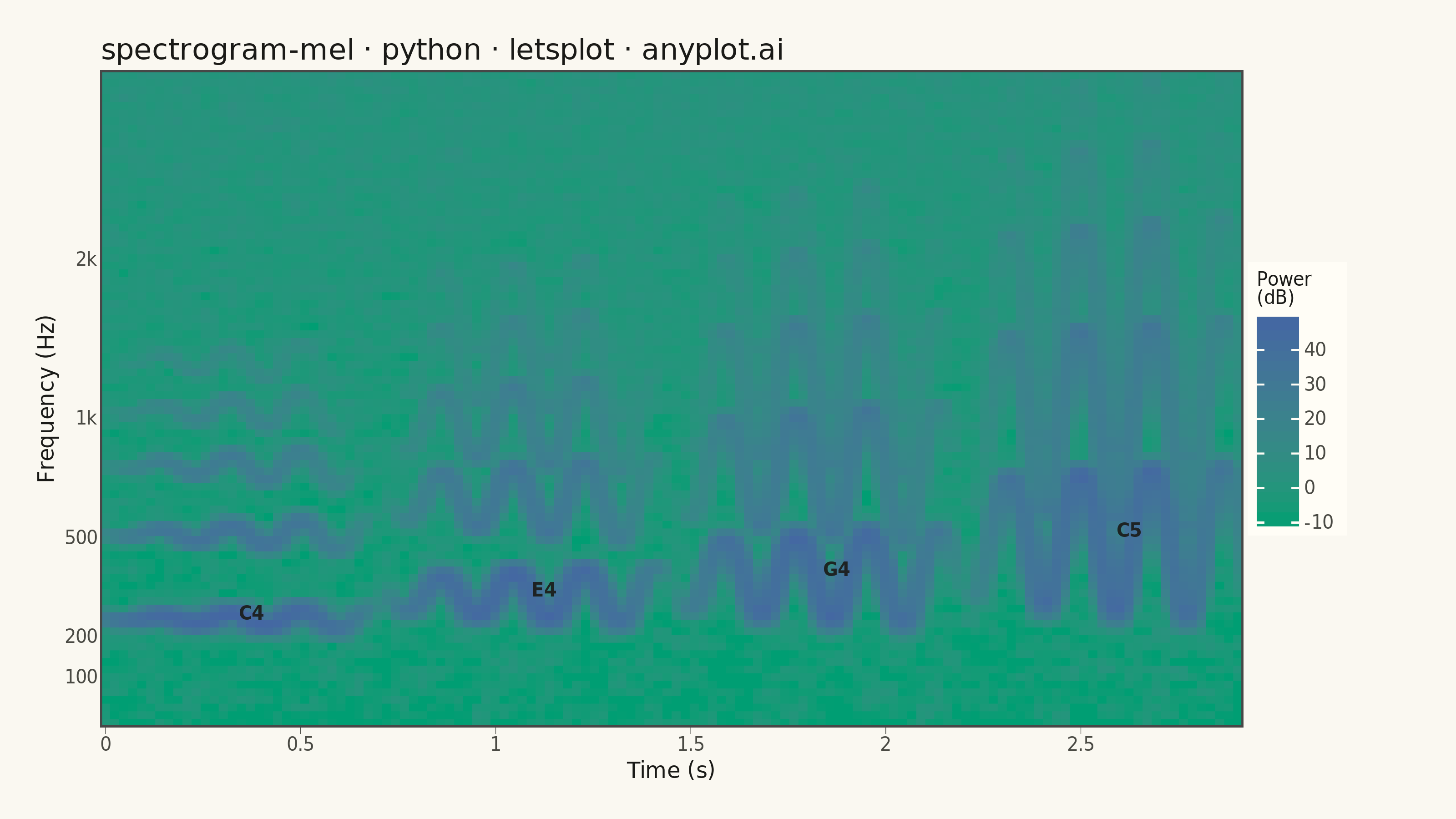
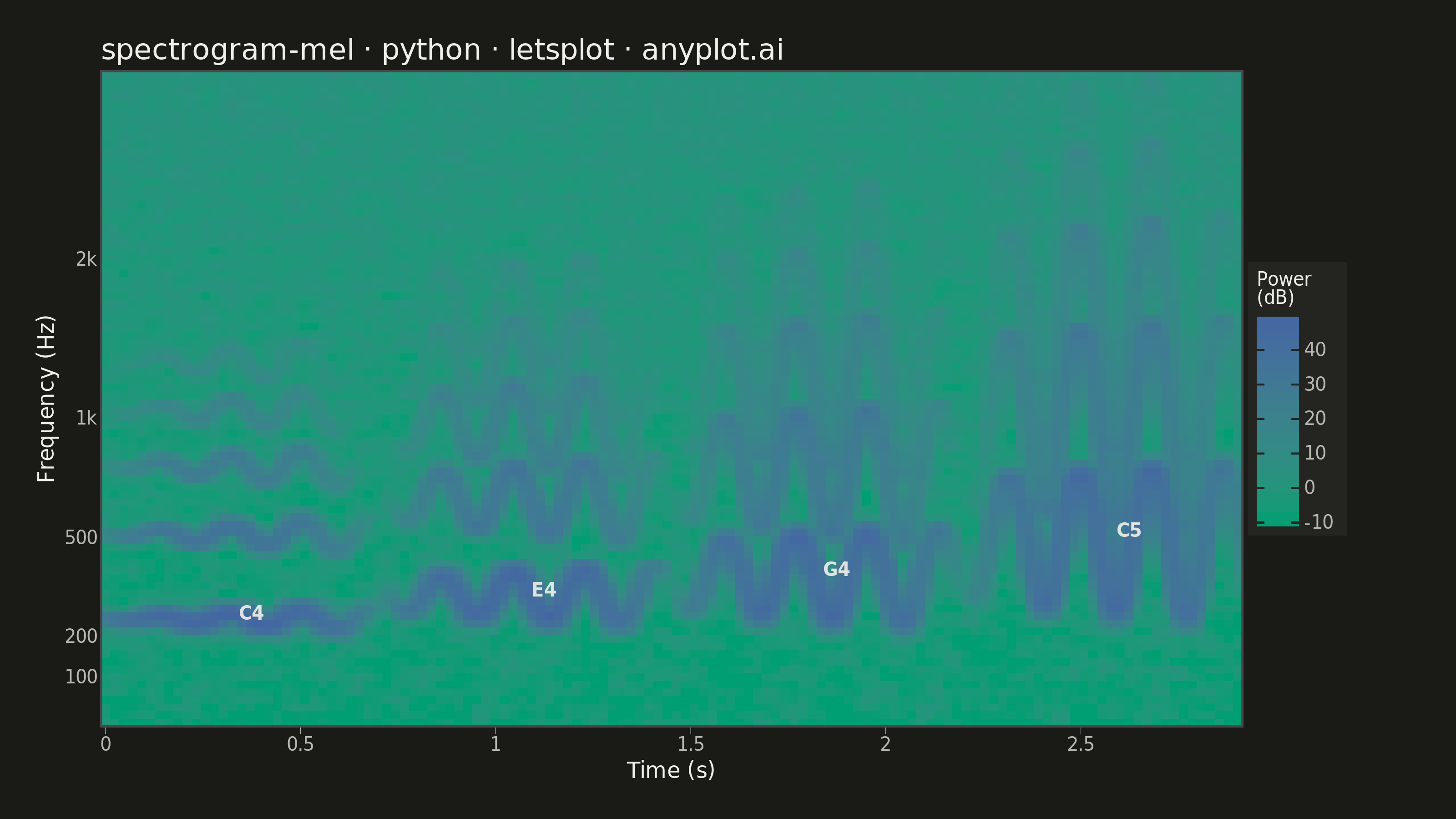
A mel-spectrogram displaying the power spectrum of an audio signal with the frequency axis warped to the mel scale, which approximates human auditory perception. Unlike a standard spectrogram with a linear frequency axis, the mel-spectrogram compresses higher frequencies and expands lower frequencies, making perceptually similar sounds visually closer together. This is the foundational input representation for modern audio machine learning pipelines including speech recognition, speaker identification, and music information retrieval.
""" anyplot.ai
spectrogram-mel: Mel-Spectrogram for Audio Analysis
Library: letsplot 4.10.1 | Python 3.13.13
Quality: 87/100 | Updated: 2026-06-03
"""

import os

import numpy as np
import pandas as pd
from lets_plot import (
    LetsPlot,
    aes,
    element_blank,
    element_line,
    element_rect,
    element_text,
    geom_text,
    geom_tile,
    ggplot,
    ggsave,
    ggsize,
    labs,
    layer_tooltips,
    scale_fill_gradient,
    scale_x_continuous,
    scale_y_continuous,
    theme,
)


LetsPlot.setup_html()

# Theme tokens — Imprint palette + theme-adaptive chrome
THEME = os.getenv("ANYPLOT_THEME", "light")
PAGE_BG = "#FAF8F1" if THEME == "light" else "#1A1A17"
ELEVATED_BG = "#FFFDF6" if THEME == "light" else "#242420"
INK = "#1A1A17" if THEME == "light" else "#F0EFE8"
INK_SOFT = "#4A4A44" if THEME == "light" else "#B8B7B0"

# Data — synthesize C major arpeggio (C4, E4, G4, C5) with harmonics and vibrato
np.random.seed(42)
sample_rate = 22050
duration = 3.0
n_samples = int(sample_rate * duration)
t = np.linspace(0, duration, n_samples, endpoint=False)

melody_freqs = [261.6, 329.6, 392.0, 523.3]
note_names = ["C4", "E4", "G4", "C5"]
audio_signal = np.zeros(n_samples)
for i, freq in enumerate(melody_freqs):
    start = int(i * n_samples / len(melody_freqs))
    end = int((i + 1) * n_samples / len(melody_freqs))
    segment_t = t[start:end]
    envelope = np.sin(np.linspace(0, np.pi, end - start)) ** 1.5
    vibrato = 1 + 0.005 * np.sin(2 * np.pi * 5.5 * segment_t)
    audio_signal[start:end] += 0.5 * envelope * np.sin(2 * np.pi * freq * vibrato * segment_t)
    for harmonic, amplitude in [(2, 0.25), (3, 0.15), (4, 0.08), (5, 0.05)]:
        audio_signal[start:end] += (
            (amplitude / harmonic) * envelope * np.sin(2 * np.pi * freq * harmonic * vibrato * segment_t)
        )

audio_signal += 0.015 * np.random.randn(n_samples)

# STFT via numpy
n_fft = 2048
hop_length = 512
n_mels = 128

window = np.hanning(n_fft)
n_frames = 1 + (n_samples - n_fft) // hop_length
stft_matrix = np.zeros((n_fft // 2 + 1, n_frames))
for frame_idx in range(n_frames):
    start_sample = frame_idx * hop_length
    frame = audio_signal[start_sample : start_sample + n_fft] * window
    spectrum = np.fft.rfft(frame)
    stft_matrix[:, frame_idx] = np.abs(spectrum) ** 2

times = np.arange(n_frames) * hop_length / sample_rate
frequencies = np.fft.rfftfreq(n_fft, 1.0 / sample_rate)

# Mel filter bank
mel_low = 2595 * np.log10(1 + 0 / 700)
mel_high = 2595 * np.log10(1 + (sample_rate / 2) / 700)
mel_points = np.linspace(mel_low, mel_high, n_mels + 2)
hz_points = 700 * (10 ** (mel_points / 2595) - 1)
fft_bins = np.floor((n_fft + 1) * hz_points / sample_rate).astype(int)

mel_filterbank = np.zeros((n_mels, len(frequencies)))
for m in range(1, n_mels + 1):
    f_left = fft_bins[m - 1]
    f_center = fft_bins[m]
    f_right = fft_bins[m + 1]
    for k in range(f_left, min(f_center, len(frequencies))):
        if f_center != f_left:
            mel_filterbank[m - 1, k] = (k - f_left) / (f_center - f_left)
    for k in range(f_center, min(f_right, len(frequencies))):
        if f_right != f_center:
            mel_filterbank[m - 1, k] = (f_right - k) / (f_right - f_center)

mel_spec = mel_filterbank @ stft_matrix
mel_spec_db = 10 * np.log10(mel_spec + 1e-10)

# Clip dB range to emphasize musical content and reduce noise floor
db_min = -10.0
db_max = float(np.max(mel_spec_db))
mel_spec_db = np.clip(mel_spec_db, db_min, db_max)

mel_center_hz = 700 * (10 ** (np.linspace(mel_low, mel_high, n_mels) / 2595) - 1)

# Downsample for tile rendering performance
time_step = max(1, len(times) // 300)
mel_step = max(1, n_mels // 128)
times_ds = times[::time_step]
mel_indices_ds = np.arange(0, n_mels, mel_step)
mel_spec_ds = mel_spec_db[::mel_step][:, ::time_step]
mel_hz_ds = mel_center_hz[mel_indices_ds]

time_grid, mel_idx_grid = np.meshgrid(times_ds, mel_indices_ds)
hz_grid = np.broadcast_to(mel_hz_ds[:, None], mel_spec_ds.shape)
df = pd.DataFrame(
    {
        "Time (s)": time_grid.flatten(),
        "Mel Band": mel_idx_grid.flatten(),
        "Power (dB)": mel_spec_ds.flatten(),
        "Freq (Hz)": hz_grid.flatten(),
    }
)

# Clamp displayed frequency range to 0–4000 Hz so harmonic content fills the canvas
df = df[df["Freq (Hz)"] <= 4000]

# Y-axis breaks: map Hz values to mel band indices
label_hz = [100, 200, 500, 1000, 2000, 4000]
label_mel_vals = [2595 * np.log10(1 + f / 700) for f in label_hz]
mel_range = np.linspace(mel_low, mel_high, n_mels)
label_indices = [float(np.interp(mv, mel_range, np.arange(n_mels))) for mv in label_mel_vals]
label_strs = ["100", "200", "500", "1k", "2k", "4k"]

# Note annotation positions (fundamental frequency of each arpeggio note)
note_annotations = []
for i, (freq, name) in enumerate(zip(melody_freqs, note_names, strict=True)):
    mel_val = 2595 * np.log10(1 + freq / 700)
    mel_idx = float(np.interp(mel_val, mel_range, np.arange(n_mels)))
    mid_time = (i + 0.5) * duration / len(melody_freqs)
    note_annotations.append({"x": mid_time, "y": mel_idx, "label": name})

df_notes = pd.DataFrame(note_annotations)

# Plot
title = "spectrogram-mel · python · letsplot · anyplot.ai"

anyplot_theme = theme(
    plot_background=element_rect(fill=PAGE_BG, color=PAGE_BG),
    panel_background=element_rect(fill=PAGE_BG),
    panel_grid_major=element_blank(),
    panel_grid_minor=element_blank(),
    axis_title=element_text(color=INK, size=12),
    axis_text=element_text(color=INK_SOFT, size=10),
    axis_line=element_line(color=INK_SOFT),
    axis_ticks=element_line(color=INK_SOFT, size=0.3),
    plot_title=element_text(color=INK, size=16),
    legend_background=element_rect(fill=ELEVATED_BG, color=INK_SOFT),
    legend_text=element_text(color=INK_SOFT, size=10),
    legend_title=element_text(color=INK, size=10),
    plot_margin=[20, 60, 20, 20],
)

plot = (
    ggplot(df, aes(x="Time (s)", y="Mel Band", fill="Power (dB)"))
    + geom_tile(
        tooltips=layer_tooltips()
        .title("Mel Spectrogram")
        .line("@{Time (s)}s | @{Freq (Hz)} Hz")
        .line("Power|@{Power (dB)} dB")
        .format("Time (s)", ".2f")
        .format("Freq (Hz)", ".0f")
        .format("Power (dB)", ".1f")
        .min_width(180)
    )
    + geom_text(aes(x="x", y="y", label="label"), data=df_notes, color=INK, size=5, fontface="bold", alpha=0.9)
    + scale_fill_gradient(low="#009E73", high="#4467A3", name="Power\n(dB)", limits=[db_min, db_max])
    + scale_y_continuous(breaks=label_indices, labels=label_strs, expand=[0, 0])
    + scale_x_continuous(expand=[0, 0])
    + labs(x="Time (s)", y="Frequency (Hz)", title=title)
    + ggsize(800, 450)
    + anyplot_theme
)

# Save
ggsave(plot, f"plot-{THEME}.png", path=".", scale=4)
ggsave(plot, f"plot-{THEME}.html", path=".")
Runnable source as JSON, for any HTTP client: https://api.anyplot.ai/specs/spectrogram-mel/letsplot/code. Any spec id and library id listed in llms-full.txt fit the same URL shape; every URL below is complete and callable.
{
  "spec_id": "spectrogram-mel",
  "language": "python",
  "library": "letsplot",
  "page": "https://anyplot.ai/spectrogram-mel/python/letsplot",
  "hub": "https://anyplot.ai/spectrogram-mel",
  "code_json": "https://api.anyplot.ai/specs/spectrogram-mel/letsplot/code",
  "spec_json": "https://api.anyplot.ai/specs/spectrogram-mel",
  "render_light_png": "https://storage.googleapis.com/anyplot-images/plots/spectrogram-mel/python/letsplot/plot-light.png",
  "render_dark_png": "https://storage.googleapis.com/anyplot-images/plots/spectrogram-mel/python/letsplot/plot-dark.png",
  "interactive_light_html": "https://storage.googleapis.com/anyplot-images/plots/spectrogram-mel/python/letsplot/plot-light.html",
  "interactive_dark_html": "https://storage.googleapis.com/anyplot-images/plots/spectrogram-mel/python/letsplot/plot-dark.html",
  "quality_score": 87.0,
  "license": "MIT",
  "guide": "https://anyplot.ai/llms.txt"
}
Part of Mel-Spectrogram for Audio Analysis on anyplot.ai.