The same plot in 14 other libraries — Python: Altair, Bokeh, lets-plot, Matplotlib, Plotly, plotnine, Pygal, Seaborn; Julia: Makie.jl; JavaScript: Chart.js, D3.js, Apache ECharts, Highcharts, MUI X Charts. Compare all 15 side by side: Spiral Time Series Chart in Python, R, Julia and JavaScript.
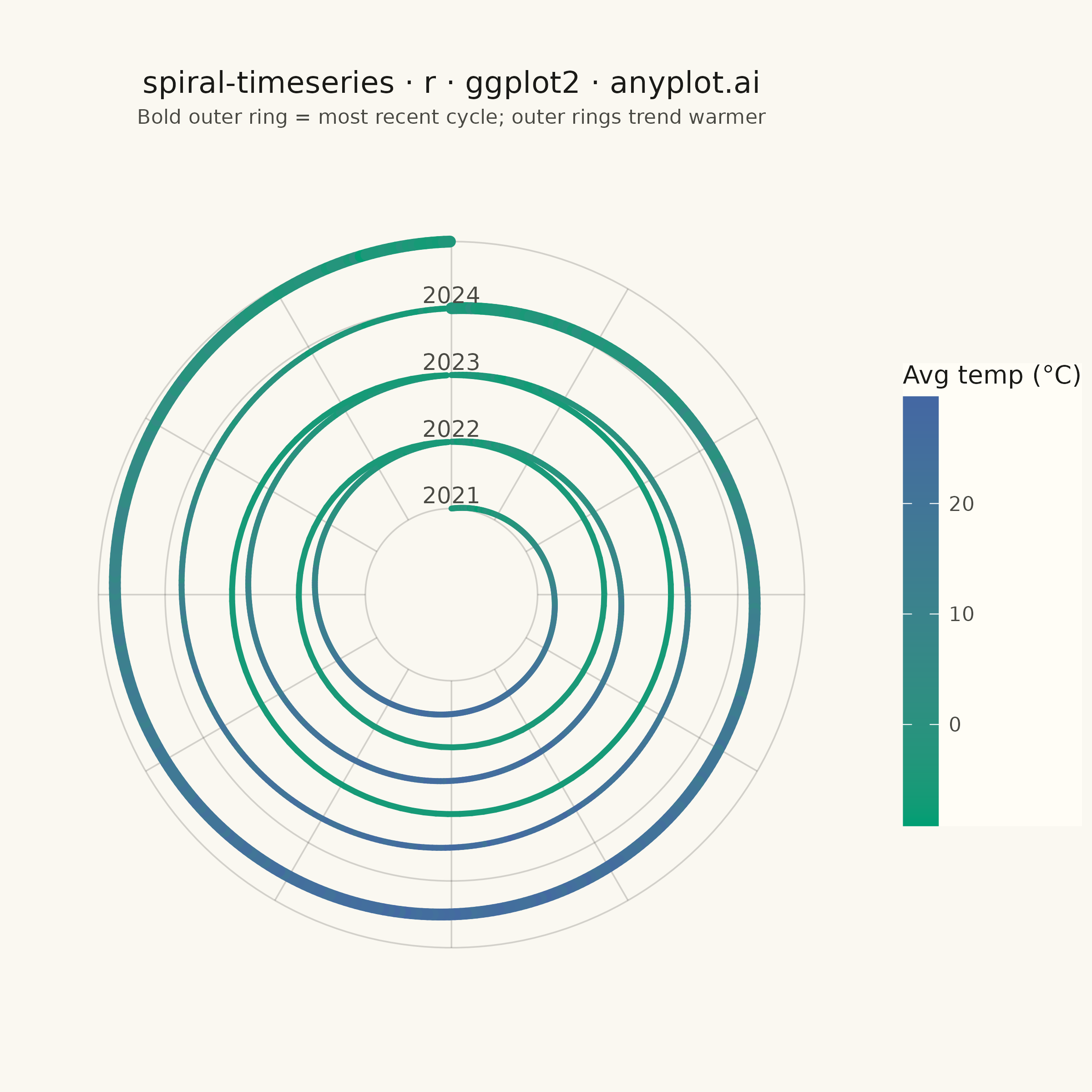
A time series plotted along a spiral (Archimedean or logarithmic), where each full revolution represents one cycle period (e.g., one year). By wrapping temporal data around a spiral, corresponding periods from different cycles align vertically, making recurring seasonal or periodic patterns immediately visible. This layout provides a compact alternative to long horizontal time series for cyclic data, revealing periodicity and trend simultaneously.
#' anyplot.ai
#' spiral-timeseries: Spiral Time Series Chart
#' Library: ggplot2 3.5.1 | R 4.4.1
#' Quality: 89/100 | Created: 2026-09-09

library(ggplot2)
library(dplyr)
library(tibble)
library(ragg)

set.seed(42)

# --- Theme tokens -------------------------------------------------------
THEME       <- Sys.getenv("ANYPLOT_THEME", "light")
PAGE_BG     <- if (THEME == "light") "#FAF8F1" else "#1A1A17"
ELEVATED_BG <- if (THEME == "light") "#FFFDF6" else "#242420"
INK         <- if (THEME == "light") "#1A1A17" else "#F0EFE8"
INK_SOFT    <- if (THEME == "light") "#4A4A44" else "#B8B7B0"
IMPRINT_PALETTE <- c("#009E73", "#C475FD", "#4467A3", "#BD8233",
                     "#AE3030", "#2ABCCD", "#954477", "#99B314")

# --- Data: daily average temperature, one revolution per year -----------
dates <- seq(as.Date("2021-01-01"), as.Date("2024-12-31"), by = "day")
years <- as.integer(format(dates, "%Y"))
doy   <- as.integer(format(dates, "%j"))

df <- tibble(
  date       = dates,
  year       = years,
  year_index = years - min(years),
  doy_frac   = (doy - 1) / 365.25
) %>%
  mutate(
    temperature = 10 - 15 * cos(2 * pi * doy_frac) +
      0.05 * year_index + rnorm(n(), mean = 0, sd = 1.8)
  )

# --- Archimedean spiral geometry (native polar coordinates) -------------
# `doy_frac` (0-1) is the theta aesthetic (one lap per cycle); `radius`
# grows by a constant GAP each lap, which is what coord_radial() renders
# as an Archimedean spiral instead of a plain circle.
R0       <- 0.6                       # inner radius (spiral start)
GAP      <- 1.0                       # radial distance added per full cycle
N_CYCLES <- max(df$year_index) + 1
r_max    <- R0 + GAP * N_CYCLES

df <- df %>%
  mutate(radius = R0 + GAP * (year_index + doy_frac))

latest_year_index <- max(df$year_index)
df_earlier <- df %>% filter(year_index < latest_year_index)
df_latest  <- df %>% filter(year_index == latest_year_index)

# Concentric rings mark each full-cycle boundary
ring_theta <- seq(0, 1, length.out = 200)
circles <- do.call(rbind, lapply(0:N_CYCLES, function(i) {
  tibble(x = ring_theta, y = R0 + GAP * i, ring = i)
}))

# Radial spokes mark month subdivisions within each cycle
month_frac <- (0:11) / 12
spokes <- tibble(x = month_frac, xend = month_frac, y = R0, yend = r_max)

# One label per revolution, at the top of the spiral, for orientation
cycle_labels <- df %>%
  distinct(year, year_index) %>%
  mutate(x = 0, y = R0 + GAP * year_index + 0.2)

# --- Title (length-scaled fontsize; see prompts/plot-generator.md) ------
plot_title <- "spiral-timeseries · r · ggplot2 · anyplot.ai"
title_size <- max(8, round(12 * min(1, 67 / nchar(plot_title))))

# --- Plot -----------------------------------------------------------------
p <- ggplot() +
  geom_path(data = circles, aes(x, y, group = ring),
            color = INK, linewidth = 0.3, alpha = 0.18) +
  geom_segment(data = spokes, aes(x = x, y = y, xend = xend, yend = yend),
               color = INK, linewidth = 0.3, alpha = 0.18) +
  geom_path(data = df_earlier, aes(x = doy_frac, y = radius, color = temperature, group = 1),
            linewidth = 1.1, lineend = "round") +
  geom_path(data = df_latest, aes(x = doy_frac, y = radius, color = temperature, group = 1),
            linewidth = 2.2, lineend = "round") +
  geom_text(data = cycle_labels, aes(x, y, label = year),
            color = INK_SOFT, size = 3.2) +
  scale_x_continuous(limits = c(0, 1)) +
  scale_y_continuous(limits = c(0, r_max)) +
  scale_color_gradient(low = IMPRINT_PALETTE[1], high = IMPRINT_PALETTE[3],
                        name = "Avg temp (°C)") +
  coord_radial(theta = "x", start = 0, end = 2 * pi,
               inner.radius = R0 / r_max, expand = FALSE) +
  labs(title = plot_title,
       subtitle = "Bold outer ring = most recent cycle; outer rings trend warmer") +
  theme_void(base_size = 8) +
  theme(
    plot.background   = element_rect(fill = PAGE_BG, color = PAGE_BG),
    panel.background  = element_rect(fill = PAGE_BG, color = NA),
    plot.title        = element_text(color = INK, size = title_size,
                                      hjust = 0.5, margin = margin(b = 4)),
    plot.subtitle     = element_text(color = INK_SOFT, size = 8,
                                      hjust = 0.5, margin = margin(b = 10)),
    legend.position    = "right",
    legend.background  = element_rect(fill = ELEVATED_BG, color = NA),
    legend.title       = element_text(color = INK, size = 10),
    legend.text        = element_text(color = INK_SOFT, size = 8),
    legend.box.spacing = unit(4, "pt"),
    plot.margin        = margin(8, 4, 2, 4)
  ) +
  guides(color = guide_colorbar(barwidth = unit(0.5, "cm"),
                                 barheight = unit(6, "cm")))

# --- Save (square canvas: symmetric radial layout) -------------------------
ggsave(
  filename = sprintf("plot-%s.png", THEME),
  plot     = p,
  device   = ragg::agg_png,
  width    = 6,
  height   = 6,
  units    = "in",
  dpi      = 400
)
Runnable source as JSON, for any HTTP client: https://api.anyplot.ai/specs/spiral-timeseries/ggplot2/code. Any spec id and library id listed in llms-full.txt fit the same URL shape; every URL below is complete and callable.
{
  "spec_id": "spiral-timeseries",
  "language": "r",
  "library": "ggplot2",
  "page": "https://anyplot.ai/spiral-timeseries/r/ggplot2",
  "hub": "https://anyplot.ai/spiral-timeseries",
  "code_json": "https://api.anyplot.ai/specs/spiral-timeseries/ggplot2/code",
  "spec_json": "https://api.anyplot.ai/specs/spiral-timeseries",
  "render_light_png": "https://storage.googleapis.com/anyplot-images/plots/spiral-timeseries/r/ggplot2/plot-light.png",
  "render_dark_png": "https://storage.googleapis.com/anyplot-images/plots/spiral-timeseries/r/ggplot2/plot-dark.png",
  "quality_score": 89.0,
  "license": "MIT",
  "guide": "https://anyplot.ai/llms.txt"
}
Part of Spiral Time Series Chart on anyplot.ai.