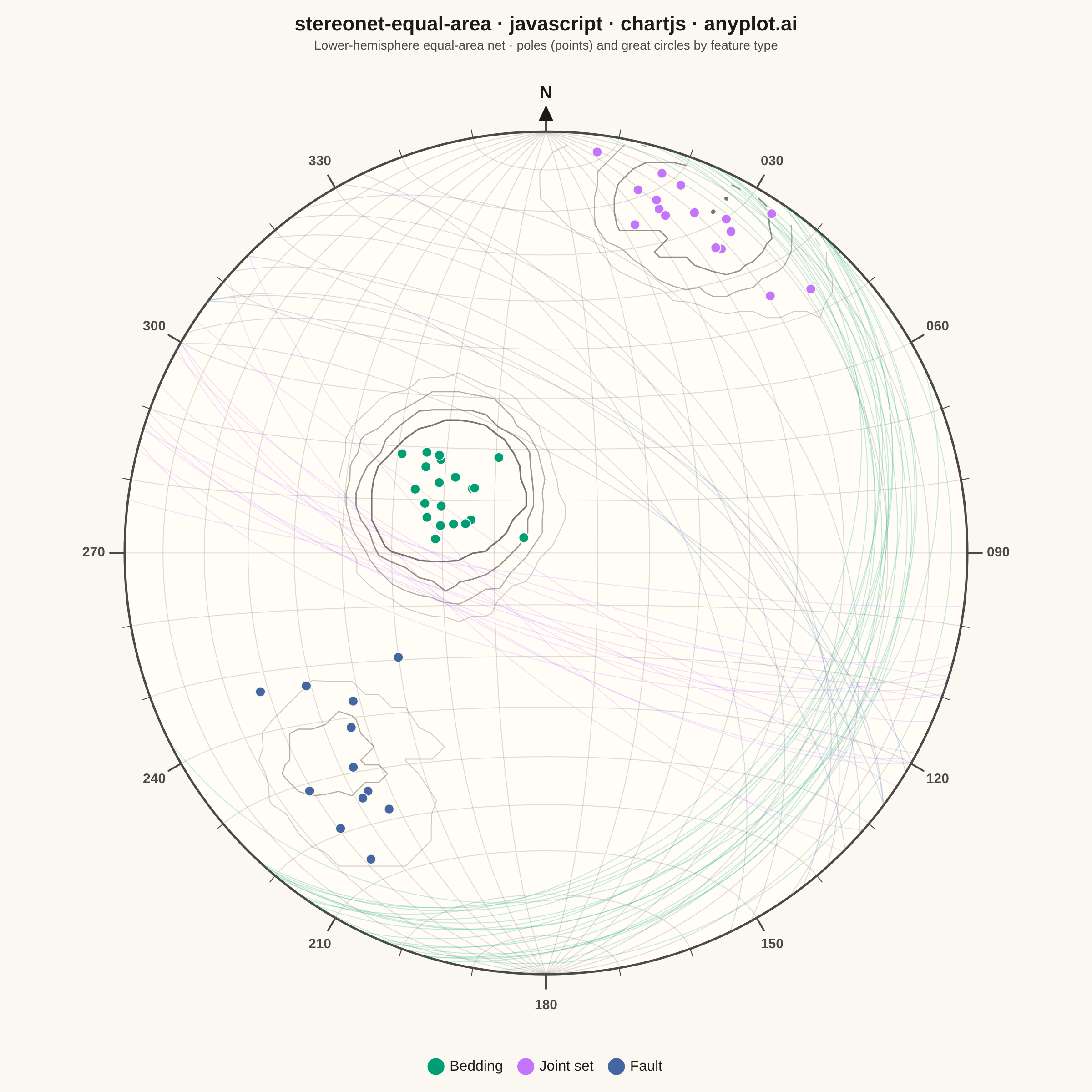
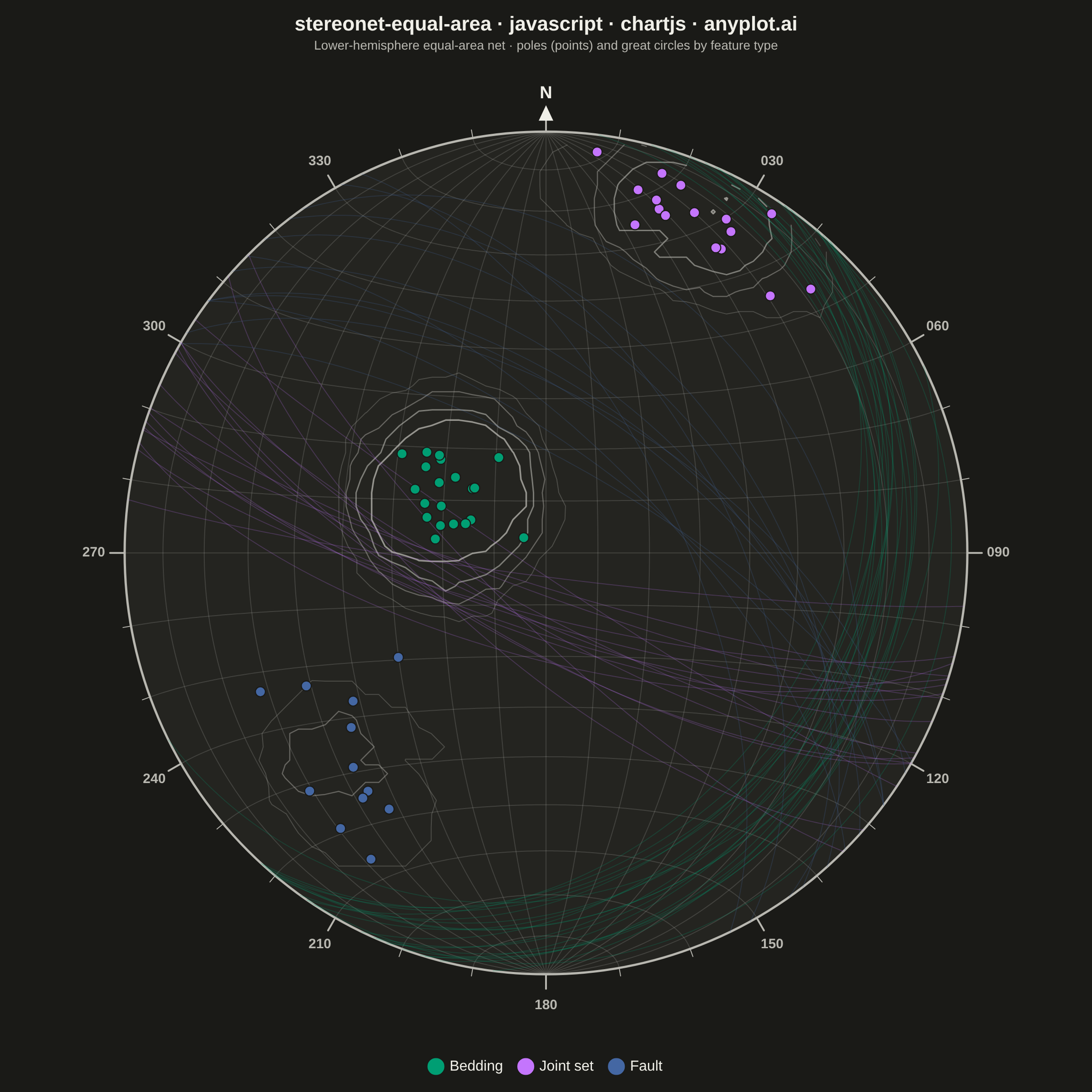
A Schmidt equal-area (lower-hemisphere) stereographic projection for plotting geological structural data. Great circles represent planar features (bedding, faults, joints) by their strike and dip, while poles to planes are plotted as points showing the orientation of the normal to each plane. Density contours highlight preferred orientations in clustered data. This is the standard projection used in structural geology for analyzing fabric elements and kinematic indicators.
// anyplot.ai
// stereonet-equal-area: Structural Geology Stereonet (Equal-Area Projection)
// Library: chartjs 4.4.7 | JavaScript 22.22.3
// Quality: 90/100 | Created: 2026-06-16
//# anyplot-orientation: square

const t = window.ANYPLOT_TOKENS;

// Theme-adaptive chrome (data colours stay constant; only chrome flips)
const PAGE = t.pageBg;
const ELEV = t.elevatedBg;
const INK = t.ink;
const INK_SOFT = t.inkSoft;
const GRID = t.grid;

// Imprint palette — bedding=brand green (first), then canonical order
const FEATURES = [
  { type: "Bedding", color: t.palette[0] }, // #009E73
  { type: "Joint set", color: t.palette[1] }, // #C475FD
  { type: "Fault", color: t.palette[2] }, // #4467A3
];

// --- Deterministic in-memory data (no RNG in the browser) -------------------
let seed = 0x2f6b3c1;
const rand = () => ((seed = (seed * 1664525 + 1013904223) >>> 0) / 4294967296);
const gauss = (mean, sd) => {
  const u1 = Math.max(rand(), 1e-9);
  const u2 = rand();
  return mean + sd * Math.sqrt(-2 * Math.log(u1)) * Math.cos(2 * Math.PI * u2);
};
const wrap360 = (a) => ((a % 360) + 360) % 360;
const clampDip = (d) => Math.max(2, Math.min(88, d));

// Each cluster mimics a field campaign: a preferred orientation plus scatter.
const CLUSTERS = [
  { feature: 0, n: 20, dipDir: 118, dip: 24, sdDir: 13, sdDip: 6 },
  { feature: 1, n: 16, dipDir: 207, dip: 79, sdDir: 9, sdDip: 6 },
  { feature: 2, n: 12, dipDir: 43, dip: 58, sdDir: 15, sdDip: 8 },
];

// Lower-hemisphere equal-area projection of a line (trend, plunge) onto the net.
const projectTP = (trendDeg, plungeDeg, cx, cy, R) => {
  const trend = (trendDeg * Math.PI) / 180;
  const zeta = ((90 - plungeDeg) * Math.PI) / 180; // colatitude from the nadir
  const r = R * Math.SQRT2 * Math.sin(zeta / 2);
  return { x: cx + r * Math.sin(trend), y: cy - r * Math.cos(trend) };
};

// Great circle of a plane given its dip direction and dip, as (trend, plunge)s.
const planeGreatCircle = (dipDirDeg, dipDeg, n = 180) => {
  const dd = (dipDirDeg * Math.PI) / 180;
  const d = (dipDeg * Math.PI) / 180;
  const sdir = ((dipDirDeg - 90) * Math.PI) / 180; // strike direction
  const u = [Math.sin(sdir), Math.cos(sdir), 0]; // strike line (horizontal)
  const v = [Math.cos(d) * Math.sin(dd), Math.cos(d) * Math.cos(dd), -Math.sin(d)]; // down-dip
  const pts = [];
  for (let i = 0; i <= n; i++) {
    const a = (Math.PI * i) / n;
    const ca = Math.cos(a);
    const sa = Math.sin(a);
    const east = ca * u[0] + sa * v[0];
    const north = ca * u[1] + sa * v[1];
    const up = ca * u[2] + sa * v[2];
    pts.push({
      trend: (Math.atan2(east, north) * 180) / Math.PI,
      plunge: (Math.asin(Math.max(-1, Math.min(1, -up))) * 180) / Math.PI,
    });
  }
  return pts;
};

const measurements = [];
CLUSTERS.forEach((c) => {
  for (let i = 0; i < c.n; i++) {
    const dipDir = wrap360(gauss(c.dipDir, c.sdDir));
    const dip = clampDip(gauss(c.dip, c.sdDip));
    measurements.push({
      feature: c.feature,
      color: FEATURES[c.feature].color,
      greatCircle: planeGreatCircle(dipDir, dip),
      poleTrend: wrap360(dipDir + 180), // pole is the plane normal
      polePlunge: 90 - dip,
    });
  }
});

// Equatorial (Schmidt) reference net: meridians (N–S striking planes dipping
// E/W) and parallels (small-circle cones about the N–S axis), every 10 degrees.
const netCurves = [];
for (let dip = 10; dip <= 80; dip += 10) {
  netCurves.push(planeGreatCircle(90, dip)); // east-dipping meridians
  netCurves.push(planeGreatCircle(270, dip)); // west-dipping meridians
}
netCurves.push(planeGreatCircle(90, 90)); // central N–S meridian
for (let alpha = 10; alpha <= 170; alpha += 10) {
  const a = (alpha * Math.PI) / 180;
  const pts = [];
  for (let i = 0; i <= 180; i++) {
    const b = (Math.PI * i) / 180;
    const east = Math.sin(a) * Math.cos(b);
    const north = Math.cos(a);
    const up = -Math.sin(a) * Math.sin(b);
    pts.push({
      trend: (Math.atan2(east, north) * 180) / Math.PI,
      plunge: (Math.asin(Math.max(-1, Math.min(1, -up))) * 180) / Math.PI,
    });
  }
  netCurves.push(pts);
};

// --- Kamb density field over the pole population ----------------------------
// Count poles inside a small counting circle at each net node, expressed in
// standard deviations above a uniform-fabric expectation (Kamb, 1959). The
// equal-area projection preserves area, so this density is meaningful.
const poleVecs = measurements.map((m) => {
  const T = (m.poleTrend * Math.PI) / 180;
  const P = (m.polePlunge * Math.PI) / 180;
  return [Math.cos(P) * Math.sin(T), Math.cos(P) * Math.cos(T), Math.sin(P)];
});
const N = poleVecs.length;
const KAMB_A = 3 / (N + 3); // counting-circle area fraction (k = 3 sigma)
const COS_RC = 1 - KAMB_A; // cos of the counting-circle angular radius
const EXP = N * KAMB_A; // expected count under a uniform fabric
const SIG = Math.sqrt(N * KAMB_A * (1 - KAMB_A));
const GN = 64; // density-grid resolution
const gridPos = Array.from({ length: GN }, (_, k) => -1 + (2 * k) / (GN - 1));
const density = new Float64Array(GN * GN);
for (let j = 0; j < GN; j++) {
  for (let i = 0; i < GN; i++) {
    const px = gridPos[i];
    const py = gridPos[j];
    const r = Math.hypot(px, py);
    if (r > 1) {
      density[j * GN + i] = NaN;
      continue;
    }
    const zeta = 2 * Math.asin(Math.min(1, r / Math.SQRT2)); // colatitude from nadir
    const trend = Math.atan2(px, -py);
    const sz = Math.sin(zeta);
    const node = [sz * Math.sin(trend), sz * Math.cos(trend), Math.cos(zeta)];
    let count = 0;
    for (let p = 0; p < N; p++) {
      const v = poleVecs[p];
      if (node[0] * v[0] + node[1] * v[1] + node[2] * v[2] >= COS_RC) count++;
    }
    density[j * GN + i] = (count - EXP) / SIG;
  }
}

// Marching squares: iso-density line segments (normalised net coords) per level.
const MS_EDGES = {
  1: [[3, 0]], 2: [[0, 1]], 3: [[3, 1]], 4: [[1, 2]],
  5: [[3, 0], [1, 2]], 6: [[0, 2]], 7: [[3, 2]], 8: [[2, 3]],
  9: [[2, 0]], 10: [[0, 1], [2, 3]], 11: [[2, 1]], 12: [[1, 3]],
  13: [[1, 0]], 14: [[0, 3]],
};
const contourSegments = (level) => {
  const segs = [];
  const edgePt = (edge, i, j, a, b, c, d) => {
    const x0 = gridPos[i];
    const x1 = gridPos[i + 1];
    const y0 = gridPos[j];
    const y1 = gridPos[j + 1];
    const lerp = (xa, ya, va, xb, yb, vb) => {
      const tt = (level - va) / (vb - va);
      return [xa + tt * (xb - xa), ya + tt * (yb - ya)];
    };
    if (edge === 0) return lerp(x0, y0, a, x1, y0, b); // top a-b
    if (edge === 1) return lerp(x1, y0, b, x1, y1, c); // right b-c
    if (edge === 2) return lerp(x1, y1, c, x0, y1, d); // bottom c-d
    return lerp(x0, y1, d, x0, y0, a); // left d-a
  };
  for (let j = 0; j < GN - 1; j++) {
    for (let i = 0; i < GN - 1; i++) {
      const a = density[j * GN + i];
      const b = density[j * GN + i + 1];
      const c = density[(j + 1) * GN + i + 1];
      const d = density[(j + 1) * GN + i];
      if (Number.isNaN(a) || Number.isNaN(b) || Number.isNaN(c) || Number.isNaN(d)) continue;
      const ci =
        (a > level ? 1 : 0) | (b > level ? 2 : 0) | (c > level ? 4 : 0) | (d > level ? 8 : 0);
      const pairs = MS_EDGES[ci];
      if (!pairs) continue;
      pairs.forEach(([e1, e2]) =>
        segs.push([edgePt(e1, i, j, a, b, c, d), edgePt(e2, i, j, a, b, c, d)]),
      );
    }
  }
  return segs;
};

// --- Helpers ----------------------------------------------------------------
const hexA = (hex, a) => {
  const n = parseInt(hex.slice(1), 16);
  return `rgba(${(n >> 16) & 255}, ${(n >> 8) & 255}, ${n & 255}, ${a})`;
};
const strokePath = (ctx, pts, cx, cy, R) => {
  ctx.beginPath();
  pts.forEach((p, i) => {
    const { x, y } = projectTP(p.trend, p.plunge, cx, cy, R);
    i === 0 ? ctx.moveTo(x, y) : ctx.lineTo(x, y);
  });
  ctx.stroke();
};

// --- Stereonet plugin: draws net, great circles and poles in pixel space ----
const stereonet = {
  id: "stereonet",
  afterDatasetsDraw(chart) {
    const { ctx, chartArea } = chart;
    const cx = (chartArea.left + chartArea.right) / 2;
    const cy = (chartArea.top + chartArea.bottom) / 2;
    const R =
      (Math.min(chartArea.right - chartArea.left, chartArea.bottom - chartArea.top) / 2) * 0.86;

    ctx.save();
    ctx.lineJoin = "round";
    ctx.lineCap = "round";

    // Net "card" so the subtle grid reads against the page surface
    ctx.beginPath();
    ctx.arc(cx, cy, R, 0, 2 * Math.PI);
    ctx.fillStyle = ELEV;
    ctx.fill();

    // Equal-area net grid (subtle)
    ctx.strokeStyle = GRID;
    ctx.lineWidth = 1;
    netCurves.forEach((c) => strokePath(ctx, c, cx, cy, R));

    // Kamb density contours — highlight preferred orientations (every 2 sigma)
    ctx.save();
    ctx.beginPath();
    ctx.arc(cx, cy, R, 0, 2 * Math.PI);
    ctx.clip();
    [2, 4, 6, 8].forEach((lv, idx) => {
      const segs = contourSegments(lv);
      if (!segs.length) return;
      ctx.strokeStyle = hexA(INK_SOFT, 0.28 + idx * 0.16);
      ctx.lineWidth = 1 + idx * 0.25;
      ctx.beginPath();
      segs.forEach(([p0, p1]) => {
        ctx.moveTo(cx + p0[0] * R, cy + p0[1] * R);
        ctx.lineTo(cx + p1[0] * R, cy + p1[1] * R);
      });
      ctx.stroke();
    });
    ctx.restore();

    // Primitive circle (the horizontal plane)
    ctx.beginPath();
    ctx.arc(cx, cy, R, 0, 2 * Math.PI);
    ctx.strokeStyle = INK_SOFT;
    ctx.lineWidth = 2.5;
    ctx.stroke();

    // Perimeter degree ticks (every 10 deg, major every 30 deg)
    ctx.fillStyle = INK_SOFT;
    ctx.font = '600 15px -apple-system, "Segoe UI", Roboto, sans-serif';
    ctx.textAlign = "center";
    ctx.textBaseline = "middle";
    for (let az = 0; az < 360; az += 10) {
      const a = (az * Math.PI) / 180;
      const dx = Math.sin(a);
      const dy = -Math.cos(a);
      const major = az % 30 === 0;
      const len = major ? 16 : 9;
      ctx.beginPath();
      ctx.moveTo(cx + R * dx, cy + R * dy);
      ctx.lineTo(cx + (R + len) * dx, cy + (R + len) * dy);
      ctx.strokeStyle = INK_SOFT;
      ctx.lineWidth = major ? 2 : 1;
      ctx.stroke();
      if (major && az !== 0) {
        ctx.fillText(String(az).padStart(3, "0"), cx + (R + len + 18) * dx, cy + (R + len + 18) * dy);
      }
    }

    // Great circles for the measured planes (faint, coloured by feature type so
    // the poles stay the focal point even where curves bunch up)
    ctx.lineWidth = 1;
    measurements.forEach((m) => {
      ctx.strokeStyle = hexA(m.color, 0.22);
      strokePath(ctx, m.greatCircle, cx, cy, R);
    });

    // Poles to planes (the primary data points)
    measurements.forEach((m) => {
      const p = projectTP(m.poleTrend, m.polePlunge, cx, cy, R);
      ctx.beginPath();
      ctx.arc(p.x, p.y, 5.5, 0, 2 * Math.PI);
      ctx.fillStyle = m.color;
      ctx.fill();
      ctx.lineWidth = 1.2;
      ctx.strokeStyle = PAGE;
      ctx.stroke();
    });

    // North arrow + label
    const ny = cy - R - 16;
    ctx.beginPath();
    ctx.moveTo(cx, ny - 13);
    ctx.lineTo(cx - 8, ny + 4);
    ctx.lineTo(cx + 8, ny + 4);
    ctx.closePath();
    ctx.fillStyle = INK;
    ctx.fill();
    ctx.font = '700 19px -apple-system, "Segoe UI", Roboto, sans-serif';
    ctx.fillText("N", cx, ny - 26);

    ctx.restore();
  },
};

// --- Mount ------------------------------------------------------------------
const canvas = document.createElement("canvas");
document.getElementById("container").appendChild(canvas);

// --- Chart ------------------------------------------------------------------
new Chart(canvas, {
  type: "scatter",
  data: { datasets: [] },
  options: {
    responsive: true,
    maintainAspectRatio: false,
    animation: false,
    layout: { padding: 10 },
    scales: {
      x: { display: false, min: -1, max: 1 },
      y: { display: false, min: -1, max: 1 },
    },
    plugins: {
      title: {
        display: true,
        text: "stereonet-equal-area · javascript · chartjs · anyplot.ai",
        color: INK,
        font: { size: 22, weight: "600" },
        padding: { top: 4, bottom: 2 },
      },
      subtitle: {
        display: true,
        text: "Lower-hemisphere equal-area net · poles (points) and great circles by feature type",
        color: INK_SOFT,
        font: { size: 14 },
        padding: { bottom: 10 },
      },
      legend: {
        position: "bottom",
        labels: {
          color: INK,
          font: { size: 16 },
          padding: 18,
          boxWidth: 14,
          boxHeight: 14,
          usePointStyle: true,
          pointStyle: "circle",
          generateLabels: () =>
            FEATURES.map((f) => ({
              text: f.type,
              fillStyle: f.color,
              strokeStyle: PAGE,
              lineWidth: 1.2,
              fontColor: INK,
            })),
        },
      },
      tooltip: { enabled: false },
    },
  },
  plugins: [stereonet],
});
Runnable source as JSON, for any HTTP client: https://api.anyplot.ai/specs/stereonet-equal-area/chartjs/code. Any spec id and library id listed in llms-full.txt fit the same URL shape; every URL below is complete and callable.
{
  "spec_id": "stereonet-equal-area",
  "language": "javascript",
  "library": "chartjs",
  "page": "https://anyplot.ai/stereonet-equal-area/javascript/chartjs",
  "hub": "https://anyplot.ai/stereonet-equal-area",
  "code_json": "https://api.anyplot.ai/specs/stereonet-equal-area/chartjs/code",
  "spec_json": "https://api.anyplot.ai/specs/stereonet-equal-area",
  "render_light_png": "https://storage.googleapis.com/anyplot-images/plots/stereonet-equal-area/javascript/chartjs/plot-light.png",
  "render_dark_png": "https://storage.googleapis.com/anyplot-images/plots/stereonet-equal-area/javascript/chartjs/plot-dark.png",
  "interactive_light_html": "https://storage.googleapis.com/anyplot-images/plots/stereonet-equal-area/javascript/chartjs/plot-light.html",
  "interactive_dark_html": "https://storage.googleapis.com/anyplot-images/plots/stereonet-equal-area/javascript/chartjs/plot-dark.html",
  "quality_score": 90.0,
  "license": "MIT",
  "guide": "https://anyplot.ai/llms.txt"
}
Part of Structural Geology Stereonet (Equal-Area Projection) on anyplot.ai.