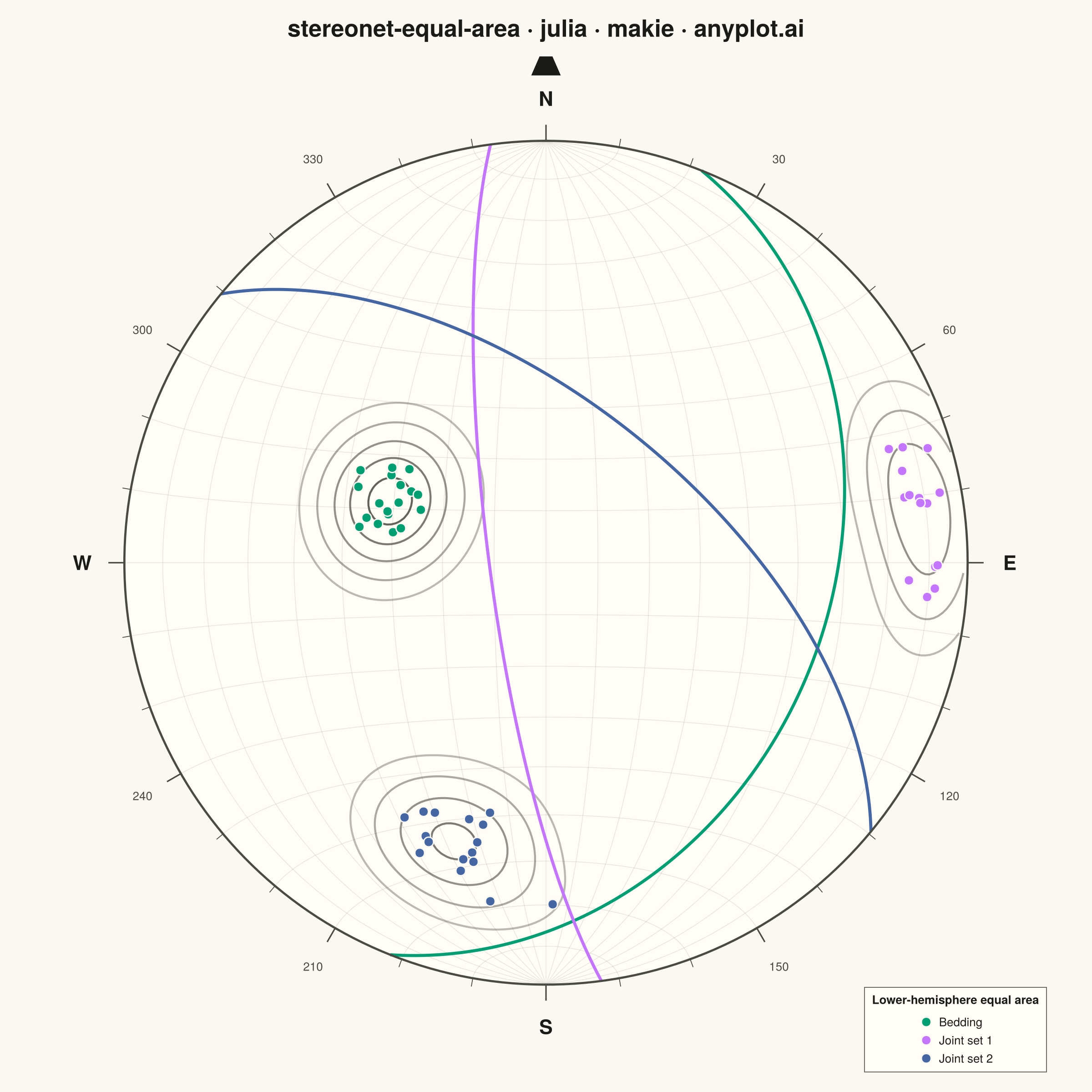
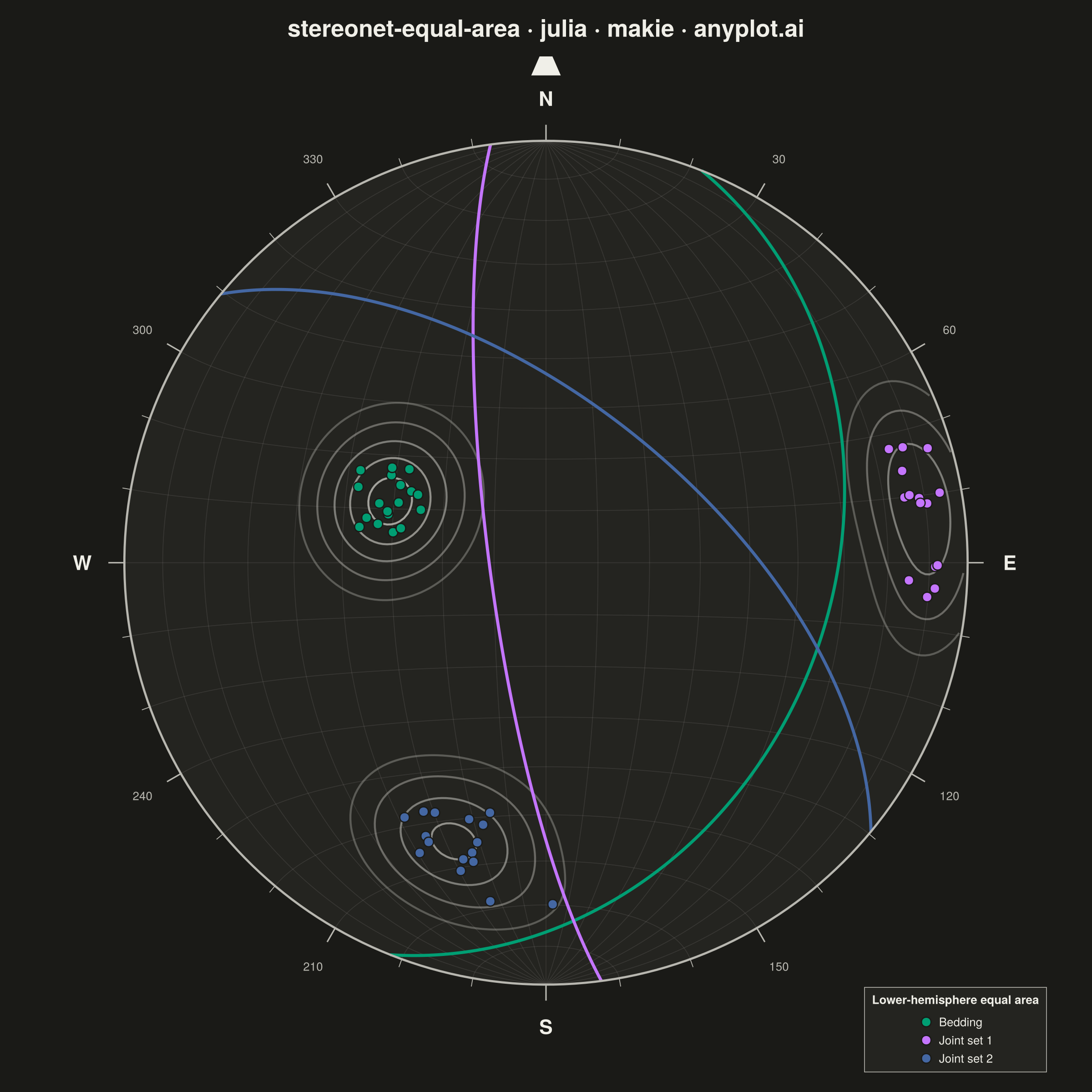
A Schmidt equal-area (lower-hemisphere) stereographic projection for plotting geological structural data. Great circles represent planar features (bedding, faults, joints) by their strike and dip, while poles to planes are plotted as points showing the orientation of the normal to each plane. Density contours highlight preferred orientations in clustered data. This is the standard projection used in structural geology for analyzing fabric elements and kinematic indicators.
# anyplot.ai
# stereonet-equal-area: Structural Geology Stereonet (Equal-Area Projection)
# Library: makie 0.22.10 | Julia 1.11.9
# Quality: 89/100 | Created: 2026-06-16

using CairoMakie
using Colors
using ColorSchemes
using Random
using Statistics

Random.seed!(42)

# --- Theme tokens -----------------------------------------------------------
const THEME       = get(ENV, "ANYPLOT_THEME", "light")
const PAGE_BG     = THEME == "light" ? colorant"#FAF8F1" : colorant"#1A1A17"
const ELEVATED_BG = THEME == "light" ? colorant"#FFFDF6" : colorant"#242420"
const INK         = THEME == "light" ? colorant"#1A1A17" : colorant"#F0EFE8"
const INK_SOFT    = THEME == "light" ? colorant"#4A4A44" : colorant"#B8B7B0"
const IMPRINT     = [
    colorant"#009E73",  # 1 — bedding (anyplot brand green)
    colorant"#C475FD",  # 2 — joint set 1 (lavender)
    colorant"#4467A3",  # 3 — joint set 2 (blue)
]
# Kamb density contours render as a single neutral ink-derived layer (varying
# alpha by level) so the density encoding reads as distinct from the colored
# feature poles rather than competing with the green/blue categorical hues.
const DENSITY_CMAP = cgrad([
    RGBAf(INK_SOFT.r, INK_SOFT.g, INK_SOFT.b, 0.28f0),
    RGBAf(INK_SOFT.r, INK_SOFT.g, INK_SOFT.b, 0.92f0),
])

# --- Equal-area projection (Schmidt net, lower hemisphere) ------------------
# A downward unit vector (E, N, D) with D >= 0 maps onto the unit disk via the
# Lambert azimuthal equal-area projection: plot_x = E / sqrt(1+D), etc.
proj_x(E, N, D) = E / sqrt(1 + D)
proj_y(E, N, D) = N / sqrt(1 + D)

# Down-positive unit vector for a line given trend (azimuth, CW from N) + plunge
line_vec(trend, plunge) =
    (sind(trend) * cosd(plunge), cosd(trend) * cosd(plunge), sind(plunge))

# Great-circle trace for a plane given dip direction + dip (lower hemisphere)
function great_circle(dip_dir, dip)
    strike = dip_dir - 90.0
    u1 = (sind(strike), cosd(strike), 0.0)                       # horizontal strike line
    u2 = line_vec(dip_dir, dip)                                  # down-dip vector
    φ  = LinRange(0.0, π, 240)
    xs = [proj_x(cos(t) * u1[1] + sin(t) * u2[1],
                 cos(t) * u1[2] + sin(t) * u2[2],
                 cos(t) * u1[3] + sin(t) * u2[3]) for t in φ]
    ys = [proj_y(cos(t) * u1[1] + sin(t) * u2[1],
                 cos(t) * u1[2] + sin(t) * u2[2],
                 cos(t) * u1[3] + sin(t) * u2[3]) for t in φ]
    return xs, ys
end

# --- Data: field measurements from a geological mapping campaign ------------
# Three structural fabric elements, each clustered around a mean orientation.
set_names = ["Bedding", "Joint set 1", "Joint set 2"]
mean_dd   = [110.0, 262.0, 18.0]    # mean dip direction (deg)
mean_dip  = [34.0, 80.0, 61.0]      # mean dip (deg)
n_obs     = [18, 15, 16]
dd_spread = [10.0, 9.0, 8.0]
dip_spread = [5.0, 4.0, 5.0]

dip_dirs = [Float64[] for _ in set_names]
dips     = [Float64[] for _ in set_names]
for s in 1:length(set_names)
    for _ in 1:n_obs[s]
        push!(dip_dirs[s], mod(mean_dd[s] + dd_spread[s] * randn(), 360.0))
        push!(dips[s], clamp(mean_dip[s] + dip_spread[s] * randn(), 2.0, 88.0))
    end
end

# Poles to planes (normals): plunge = 90 - dip, trend = dip_dir + 180
pole_xy  = [Tuple{Float64,Float64}[] for _ in set_names]
pole_vec = NTuple{3,Float64}[]      # flat list of all pole vectors for density
for s in 1:length(set_names)
    for k in 1:n_obs[s]
        v = line_vec(dip_dirs[s][k] + 180.0, 90.0 - dips[s][k])
        push!(pole_xy[s], (proj_x(v...), proj_y(v...)))
        push!(pole_vec, v)
    end
end

# --- Kamb-style density field over the projection disk ----------------------
# Each grid node is back-projected to a downward unit vector; density is the
# sum of a smoothing kernel over all poles (counts preferred orientations).
ng   = 200
grid = LinRange(-1.0, 1.0, ng)
ksm  = 45.0                          # counting-cone concentration
density = fill(NaN, ng, ng)
for i in 1:ng, j in 1:ng
    gx, gy = grid[i], grid[j]
    ρ2 = gx^2 + gy^2
    ρ2 > 1.0 && continue
    D = 1.0 - ρ2                      # inverse equal-area projection
    f = sqrt(2.0 - ρ2)
    gE, gN, gD = gx * f, gy * f, D
    acc = 0.0
    for (pE, pN, pD) in pole_vec
        acc += exp(ksm * (gE * pE + gN * pN + gD * pD - 1.0))
    end
    density[i, j] = acc
end
dmax    = maximum(filter(!isnan, density))
density ./= dmax
levels  = [0.15, 0.30, 0.50, 0.70, 0.90]

# --- Figure (square — the stereonet has no preferred horizontal axis) -------
fig = Figure(size = (1200, 1200), fontsize = 14, backgroundcolor = PAGE_BG)

ax = Axis(
    fig[1, 1];
    title                = "stereonet-equal-area · julia · makie · anyplot.ai",
    titlesize            = 26,
    titlecolor           = INK,
    titlegap             = 16,
    aspect               = DataAspect(),
    backgroundcolor      = PAGE_BG,
    xgridvisible         = false,
    ygridvisible         = false,
    xticksvisible        = false,
    yticksvisible        = false,
    xticklabelsvisible   = false,
    yticklabelsvisible   = false,
    leftspinevisible     = false,
    rightspinevisible    = false,
    topspinevisible      = false,
    bottomspinevisible   = false,
)
limits!(ax, -1.20, 1.20, -1.22, 1.20)

# Elevated disk so the net sits on a subtly distinct surface
disk_θ = LinRange(0, 2π, 256)
poly!(ax, Point2f.(cos.(disk_θ), sin.(disk_θ)); color = ELEVATED_BG, strokewidth = 0)

# Net graticule: meridians + small circles every 10° (subtle reference grid)
net_col = RGBAf(INK.r, INK.g, INK.b, 0.10f0)
for λ in -80.0:10.0:80.0                 # meridians (great circles about N–S axis)
    φ = LinRange(-90.0, 90.0, 180)
    xs = [proj_x(cosd(p) * sind(λ), sind(p), cosd(p) * cosd(λ)) for p in φ]
    ys = [proj_y(cosd(p) * sind(λ), sind(p), cosd(p) * cosd(λ)) for p in φ]
    lines!(ax, xs, ys; color = net_col, linewidth = 0.8)
end
for φ0 in -80.0:10.0:80.0                # parallels (small circles)
    λ = LinRange(-90.0, 90.0, 180)
    xs = [proj_x(cosd(φ0) * sind(l), sind(φ0), cosd(φ0) * cosd(l)) for l in λ]
    ys = [proj_y(cosd(φ0) * sind(l), sind(φ0), cosd(φ0) * cosd(l)) for l in λ]
    lines!(ax, xs, ys; color = net_col, linewidth = 0.8)
end

# Kamb density contours — highlight preferred pole orientations
contour!(ax, grid, grid, density;
    levels = levels, colormap = DENSITY_CMAP, linewidth = 2.2)

# Mean great circle per fabric element (representative plane)
for s in 1:length(set_names)
    xs, ys = great_circle(mean(dip_dirs[s]), mean(dips[s]))
    lines!(ax, xs, ys; color = IMPRINT[s], linewidth = 3.4)
end

# Poles to planes, colored by fabric element (one labeled scatter per set)
for s in 1:length(set_names)
    px = [p[1] for p in pole_xy[s]]
    py = [p[2] for p in pole_xy[s]]
    scatter!(ax, px, py;
        color = IMPRINT[s], markersize = 15, strokecolor = PAGE_BG,
        strokewidth = 1.4, label = set_names[s])
end

# Primitive circle (horizontal plane / perimeter)
lines!(ax, cos.(disk_θ), sin.(disk_θ); color = INK_SOFT, linewidth = 2.4)

# Perimeter degree ticks every 10°; cardinal + azimuth labels
for az in 0.0:10.0:350.0
    major = az % 30 == 0
    r2 = major ? 1.038 : 1.020
    lines!(ax, [sind(az), sind(az) * r2], [cosd(az), cosd(az) * r2];
        color = INK_SOFT, linewidth = major ? 1.6 : 0.9)
end
for az in 0.0:30.0:330.0
    cardinal = az == 0 ? "N" : az == 90 ? "E" : az == 180 ? "S" : az == 270 ? "W" : nothing
    if cardinal === nothing
        text!(ax, sind(az) * 1.105, cosd(az) * 1.105;
            text = string(Int(az)), fontsize = 13, color = INK_SOFT,
            align = (:center, :center))
    else
        text!(ax, sind(az) * 1.10, cosd(az) * 1.10;
            text = cardinal, fontsize = 22, color = INK, font = :bold,
            align = (:center, :center))
    end
end

# North arrow above the primitive circle
poly!(ax, Point2f[(-0.035, 1.155), (0.035, 1.155), (0.0, 1.235)];
    color = INK, strokewidth = 0)

axislegend(ax, "Lower-hemisphere equal area";
    position        = :rb,
    backgroundcolor = ELEVATED_BG,
    labelcolor      = INK,
    titlecolor      = INK,
    framecolor      = INK_SOFT,
    framewidth      = 0.8,
    labelsize       = 13,
    titlesize       = 13,
    patchsize       = (18, 18),
    padding         = (8, 8, 6, 6),
    margin          = (6, 6, 6, 6),
    rowgap          = 2,
)

# --- Save -------------------------------------------------------------------
save("plot-$(THEME).png", fig; px_per_unit = 2)
Runnable source as JSON, for any HTTP client: https://api.anyplot.ai/specs/stereonet-equal-area/makie/code. Any spec id and library id listed in llms-full.txt fit the same URL shape; every URL below is complete and callable.
{
  "spec_id": "stereonet-equal-area",
  "language": "julia",
  "library": "makie",
  "page": "https://anyplot.ai/stereonet-equal-area/julia/makie",
  "hub": "https://anyplot.ai/stereonet-equal-area",
  "code_json": "https://api.anyplot.ai/specs/stereonet-equal-area/makie/code",
  "spec_json": "https://api.anyplot.ai/specs/stereonet-equal-area",
  "render_light_png": "https://storage.googleapis.com/anyplot-images/plots/stereonet-equal-area/julia/makie/plot-light.png",
  "render_dark_png": "https://storage.googleapis.com/anyplot-images/plots/stereonet-equal-area/julia/makie/plot-dark.png",
  "quality_score": 89.0,
  "license": "MIT",
  "guide": "https://anyplot.ai/llms.txt"
}
Part of Structural Geology Stereonet (Equal-Area Projection) on anyplot.ai.